Comparisons between real and simulated data

In order to assess the efficiency of the detector, a number of monoenergetic sources were simulated in a no scattering environment in order to calculate a simulated efficiency of capture on \(^{6}\)Li:ZnS. This data was then compared with real data taken at NPL, with known incident fluence, to ensure that the simulated efficiency is consistent with a real efficiency.

Initially there was a discrepancy between the simulated efficiency and the real efficiency that was inconsistent between the 144 keV and 1.2 MeV measurements at NPL; the real efficiency at 144 keV was ~10% less than the simulated efficiency at the same energy, whereas the 1.2 MeV real efficiency was consistent with the simulated efficiency at that energy within 1\(\sigma\). This can be seen in Figure 1, below.

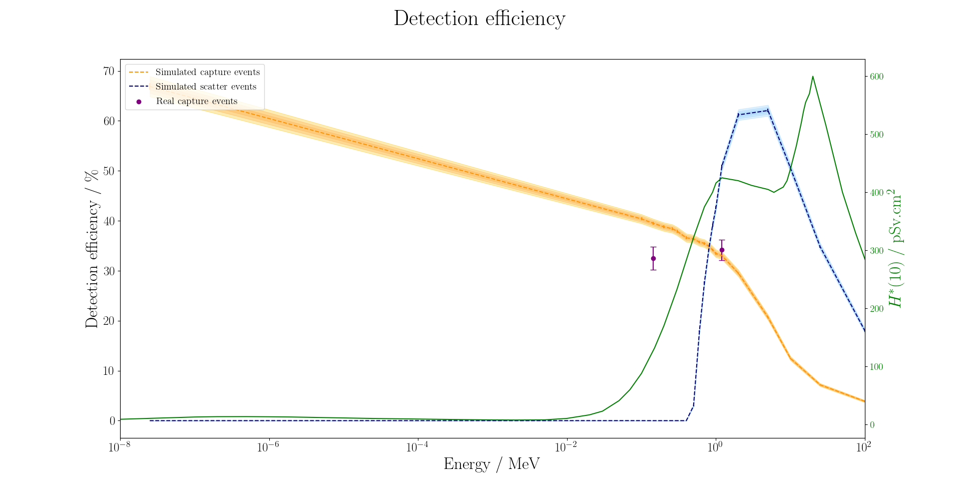Figure 1: Original capture efficiency plot. The inconsistency between real and simulated efficiency at the two different real data energies suggests some unaccounted-for effect in either the real calculation or the simulated calculation.

In order to investigate this discrepancy it is informative to compare the cube-level rates for the real data and the simulated data, to see if the discrepancy is due to a physical effect in some specific cubes. Thse comparisons can be seen in Figure 2 and Figure 3, along with the fractional difference between the two datasets.

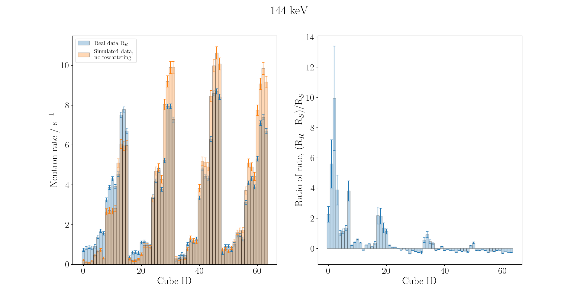Figure 2: Left: cube-level comparison between shadowcone-subtracted real data and simulated data for 144 keV. Right: fractional difference between shadowcone-subtracted real and simulated datasets.

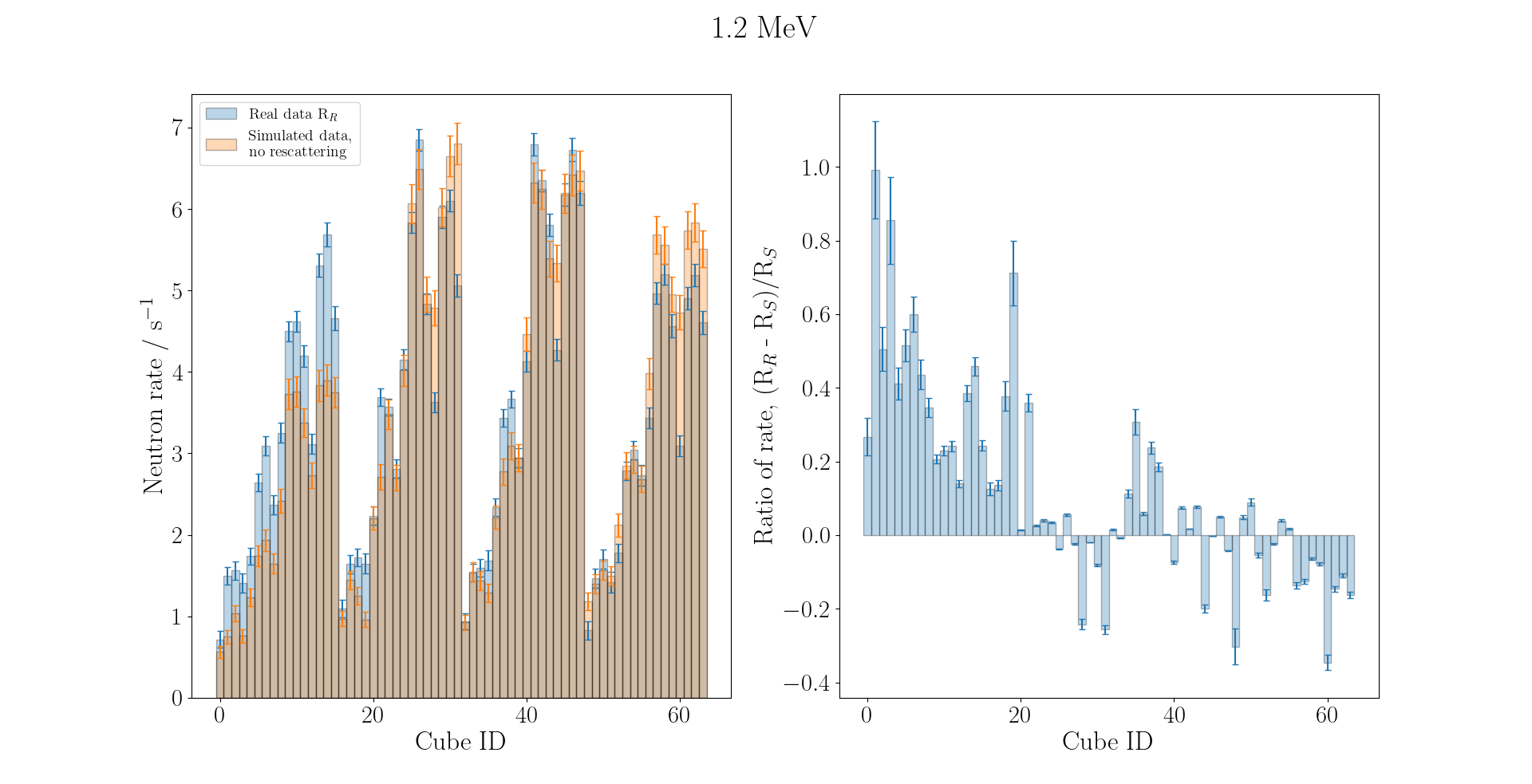Figure 3: Left: Cube-level comparison between shadowcone-subtracted real data and simulated data for 1.2 MeV. Right: fractional difference between shadowcone-subtracted real and simulated datasets.

The source of increased count for the first 16 cubes can be identified by looking at the y and z coordinates associated with these cubes, as shown in Figure 4. These cubes all lie in the Z = 0 plane, so the real excess is on the bottom face of the detector. This is due to neutrons scattering out of the bottom face of the detector, but then scattering back into the detector, off of the stand the detector was resting on. This effect is not present in the simulated data set as the stand was not simulated. We also note an excess some Y = 0 cubes, attributed to scattering off of the back wall.

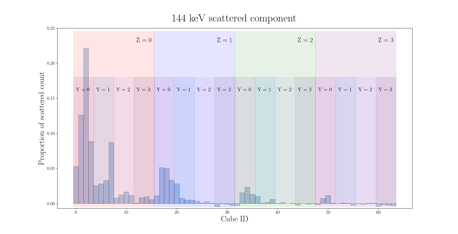Figure 4: Distribution of the scattered count for 144 keV, with cubes labelled by y and z coordinates. The excess in the Z = 0 and Y = 0 cubes is from scattering on the stand and back wall.

Firstly, the shadowcone measurements for both energies were examined to ensure that the scattered component was consistent for both incident neutron energies. This was also done to check that the shadowcone subtraction was being performed correctly and consistently for both energies. The 3D view of the two shadowcone measurements can be seen in Figure 5, and the cube level comparison can be seen in Figure 6.

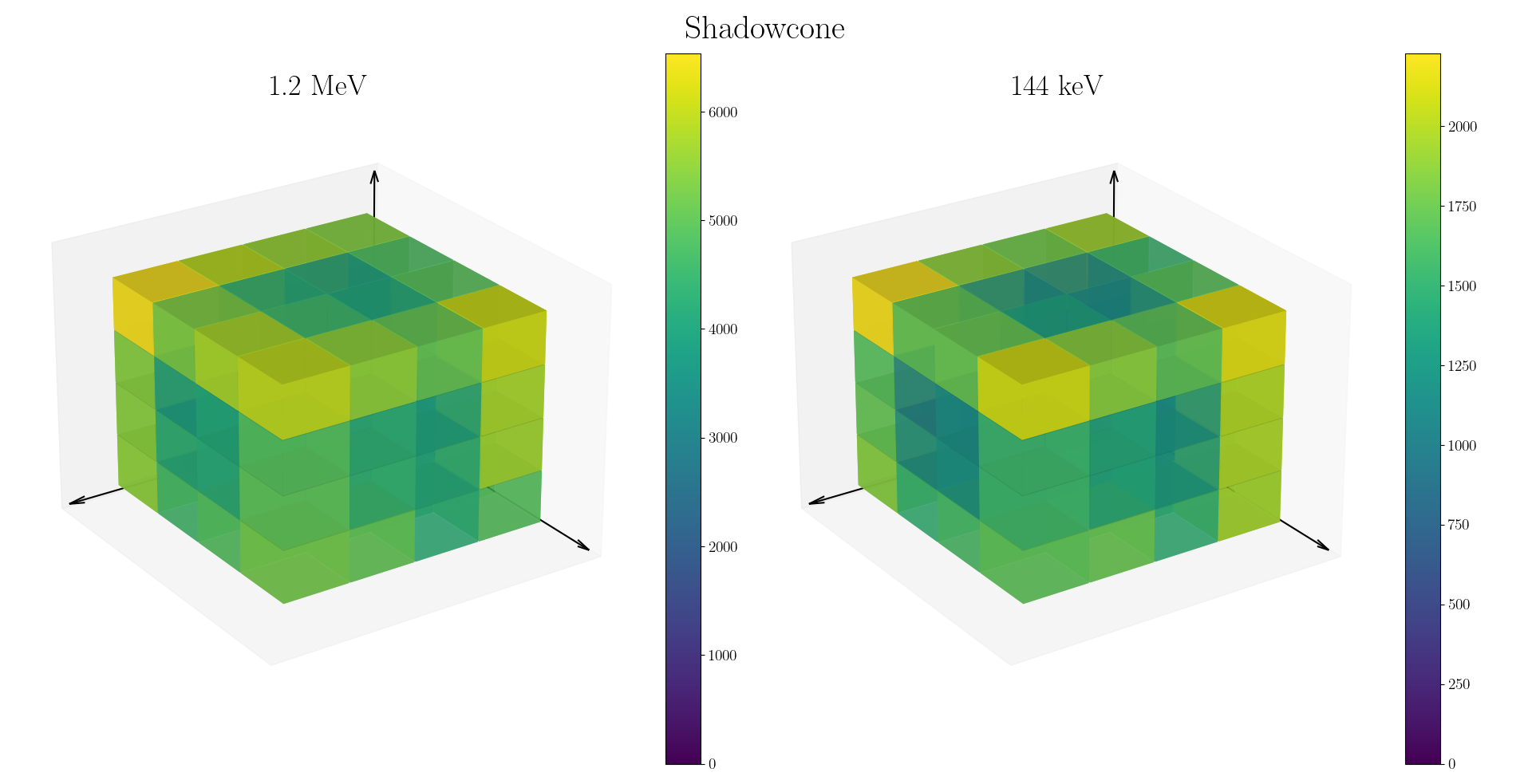
Figure 5: 3D view of shadowcone measurements, to ensure the shadowcone distribution is consistent between runs.

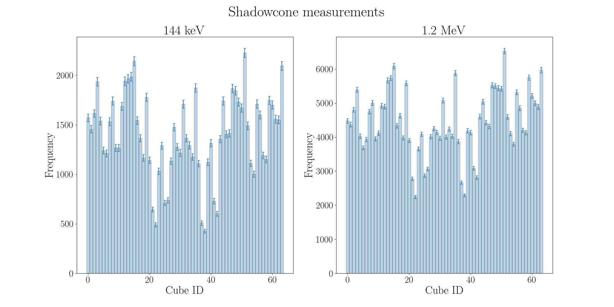
Figure 6: Cube level counts in each shadowcone dataset.

From these plots, we can see the shape of the distribution is very similar between the two datasets. After calculating the fraction of count per cube, the mean absolute deviation between the 144 keV and 1.2 MeV datasets is 11.6 \(\pm\) 0.6 %. These differences are attributed to the different initial neutron energy resulting in e.g. additional scatters for the 1.2 MeV neutrons than for the 144 keV neutrons.

Further inspection of the shadowcone subtraction method revealed an error introduced by the variation of fluence between the shadowcone and full exposure measurements. To compensate for this, the shadowcone and full exposure measurements were normalised to the same incident fluence and exposure time before subtraction, whereas before they were only normalised by exposure time. As a result there is another contribution to the uncertainty on each cube rate, from the uncertainty on the fluence measurement provided by NPL.

PROVIDE DETAILS OF CALCULATION FOR COMPARISON

The updated comparison between real and simulated data for both cases can be seen in Figures 7 and 8.

Figure 7: Comparison between real shadowcone-subtracted data and simulated data for 144 keV neutrons following the correction to the shadowcone subtraction.

Figure 8: Comparison between real shadowcone-subtracted data and simulated data for 1.2 MeV neutrons following the correction to the shadowcone subtraction.

From these figures, it is clear that this does not account for the discrepancy. Subsequently, the simulated data was analysed with the detector at 1.5 m and at 4.33 m in the 144 keV case, and at 1.5 m and 4.85 m in the 1.2 MeV case (the simulation reference distance and the real NPL measurement distance respectively). This was done to look for any air-scattering effects that could contribute to the discrepancy found.

Firstly, the fraction of acceptance occupied by the detector was calculated in all cases. The simulation was configured to emit neutrons in a cone around the negative y-axis with a half-angle of 15\(^{\circ}\). The detector was positioned such that the front face at the detector was at -\(d\) for desired distance \(d\), so neutrons were incident on Y = 3 face as in the NPL exercise. The fraction of acceptance was calculated by taking the ratio of the surface area of the detector facing the source, \(A_D\) and the total surface area subtended at the surface of the detector by the cone of neutron emission, \(A_E\). This fraction \(F_A\) is then defined as

\[F_A = \frac{A_D}{A_E}.\]

The other key ratio is the fraction of the generated neutrons incident on the detector in the simulation \(F_C\), defined as

\[F_C = \frac{C_I}{C_G},\]

for incident count \(C_I\) and generated count \(C_G\). By comparing the ratio \(F_C/F_A\) at the two distances, we can see what effect there is from air scattering. These values are summarised below in Table 1, alongside the calculated simulated capture effficiency.

Energy	Distance	Incident count C\(_I\)	Generated count C\(_G\)	Fraction of generated count incident F\(_C\) = C\(_I\)/C:math:_G	Fraction of acceptance F\(_A\)	Ratio F\(_C\) / F\(_A\)	Captured count C\(_C\)	Capture Efficiency C\(_C\)/C:math:_I
144 keV	1.5 m	237395 \(\pm\) 487	4000000	0.0593 \(\pm\) 0.0001	0.0830	0.715 \(\pm\) 0.001	94161 \(\pm\) 307	0.397 \(\pm\) 0.002
	4.33 m	27907 \(\pm\) 167	4000000	0.00698 \(\pm\) 0.00004	0.00997	0.700 \(\pm\) 0.004	11173 \(\pm\) 106	0.400 \(\pm\) 0.004
1.2 MeV	1.5 m	268708 \(\pm\) 518	4000000	0.0672 \(\pm\) 0.0001	0.0830	0.809 \(\pm\) 0.002	89546 \(\pm\) 299	0.333 \(\pm\) 0.001
	4.85 m	25662 \(\pm\) 160	4000000	0.00642 \(\pm\) 0.00004	0.00794	0.808 \(\pm\) 0.005	8707 \(\pm\) 93	0.339 \(\pm\) 0.004

Table 1: comparison of \(F_C\) and \(F_A\) to determine the effect of air scattering in the simulation. We note a reduction in the ratio \(F_C\)/\(F_A\) of 2.1% for 144 keV and of 0.1% for 1.2 MeV, when moving from 1.5 m to the far distance of 4.33 / 4.85 m respectively.

From this comparison, we find that the air scattering effect difference between the two distances is 2.1% in the 144 keV case and 0.1% in the 1.2 MeV case, and therefore not sufficient to explain the discrepancy bewteen the shadowcone-subtracted real data and the simulated data. However, the comparison of \(F_C\)/\(F_A\) for 144 keV and 1.2 MeV reveals an energy-dependent discrepancy between the two; by considering just the 1.5 m case, the fraction of acceptance \(F_A\) is constant and therefore this discrepancy must lie in the fraction of generated count that is incident on the detector, \(F_C\). This prompted investigation into the method of calculating count incident on the detector face.

The initial calculation of incident count looked for any simulated neutrons that entered the active volume of the detector, which consisted of the volume occupied by the PVT cubes and the LiF:ZnS screens. However, this is not equivalent to the incidence considered in the NPL exercise, which is the case of the detector. It is then hypothesised that this discrepancy is resulting from scattering on the case of the detector resulting in more neutrons being scattered out of the detector in the 144 keV case than in the 1.2 MeV case.

After correction of the incident count, the discrepancy betweeen 144 keV and 1.2 MeV is greatly reduced and they are now consistent with each other within 2\(\sigma\) when comparing the 4.33 m and 4.85 m cases. This can be seen in Table 2. It is worth noting that the ratio \(F_C\)/\(F_A\) is not equal to one, as might be expected; this is expected to be due to the fraction of acceptance comparing a flat, square surface to a curved spherical cap.

Energy	Distance	Incident count C\(_I\)	Generated count C\(_G\)	Fraction of generated count incident F\(_C\) = C\(_I\)/C:math:_G	Fraction of acceptance F\(_A\)	Ratio F\(_C\) / F\(_A\)	Captured count C\(_C\)	Capture Efficiency C\(_C\)/C:math:_I
144 keV	4.33 m	31489 \(\pm\) 177	4000000	0.00787 \(\pm\) 0.00004	0.00997	0.790 \(\pm\) 0.004	11173 \(\pm\) 106	0.355 \(\pm\) 0.004
1.2 MeV	4.85 m	25690 \(\pm\) 160	4000000	0.00642 \(\pm\) 0.00004	0.00794	0.809 \(\pm\) 0.005	8707 \(\pm\) 93	0.339 \(\pm\) 0.004

Table 2: comparison of \(F_C\) and \(F_A\) following update to the calculation of incident count. The value of \(F_C\)/\(F_A\) for the two energies is now consistent at the 2\(\sigma\) level.

Now that this discrepancy between the two energies has been resolved, the simulated data at the cube level can again be compared with the real data. These comparisons can be seen in Figure 9.

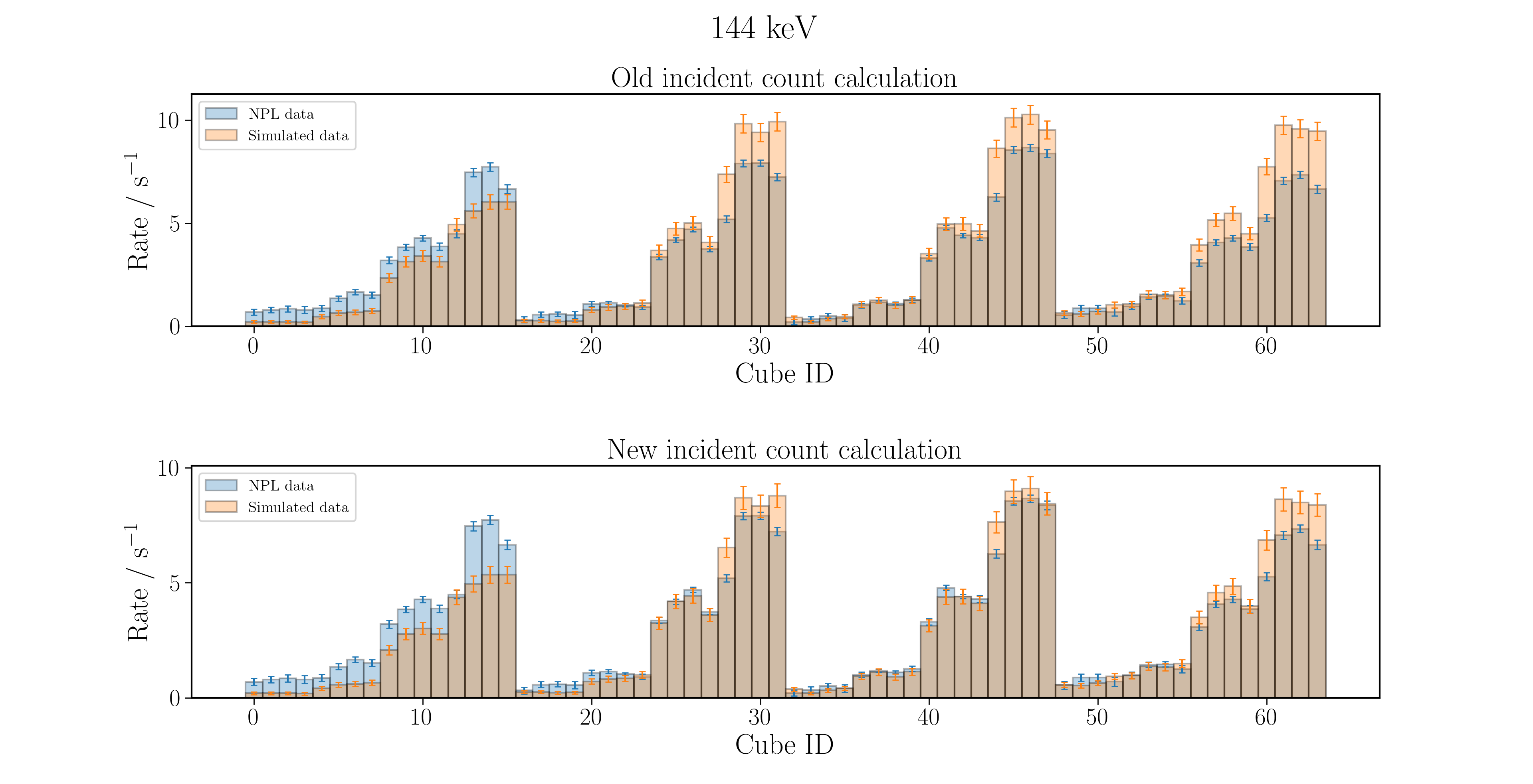
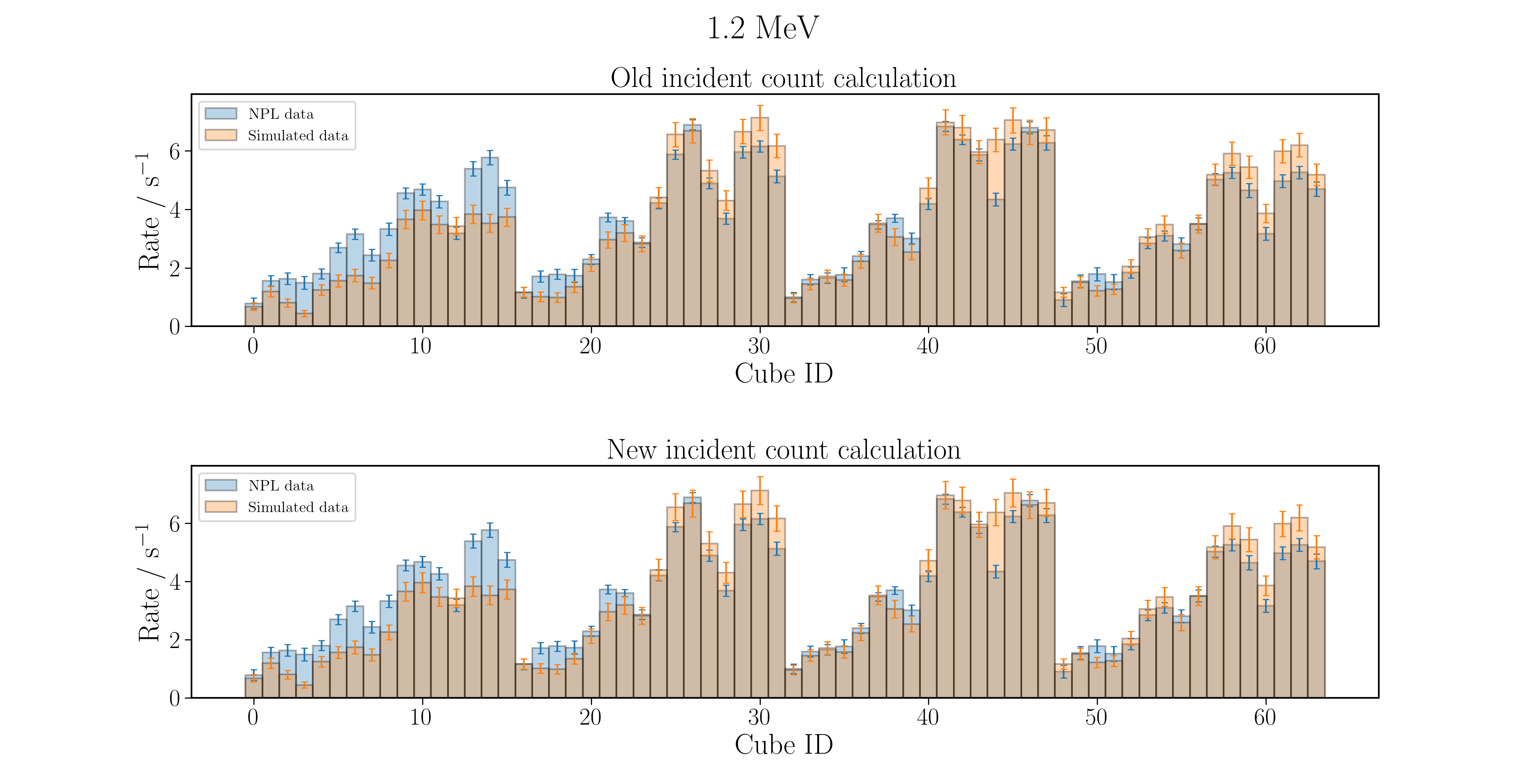
Figure 9: Comparison between real and simulated cube-level rates for 144 keV (a) and 1.2 MeV (b), for both the old incident count calculation and the new calculation. For 144 keV, the agreement is greatly improved with the new calculation for Cube ID greater than 16. For Cube ID less than 16 the discrepancy is attributed to an excess of real counts from scattering on the stand the detector was resting on, in both cases.

From this comparison we can see that the 144 keV dataset is now in much better agreement with the real data for the majority of cubes, and that the excess of real counts for Cube ID less than 16 is consistent with the corresponding excess with the 1.2 MeV dataset. This excess is attributed to neutrons scattering out of the bottom of the detector, then scattering off of the stand the detector was resting on and back into the detector.

Now that this comparison has been validated, the simulated efficiency can be recalculated to check that the real efficiency is now consistent with the simulated efficiency. This can be seen in Figure 10.

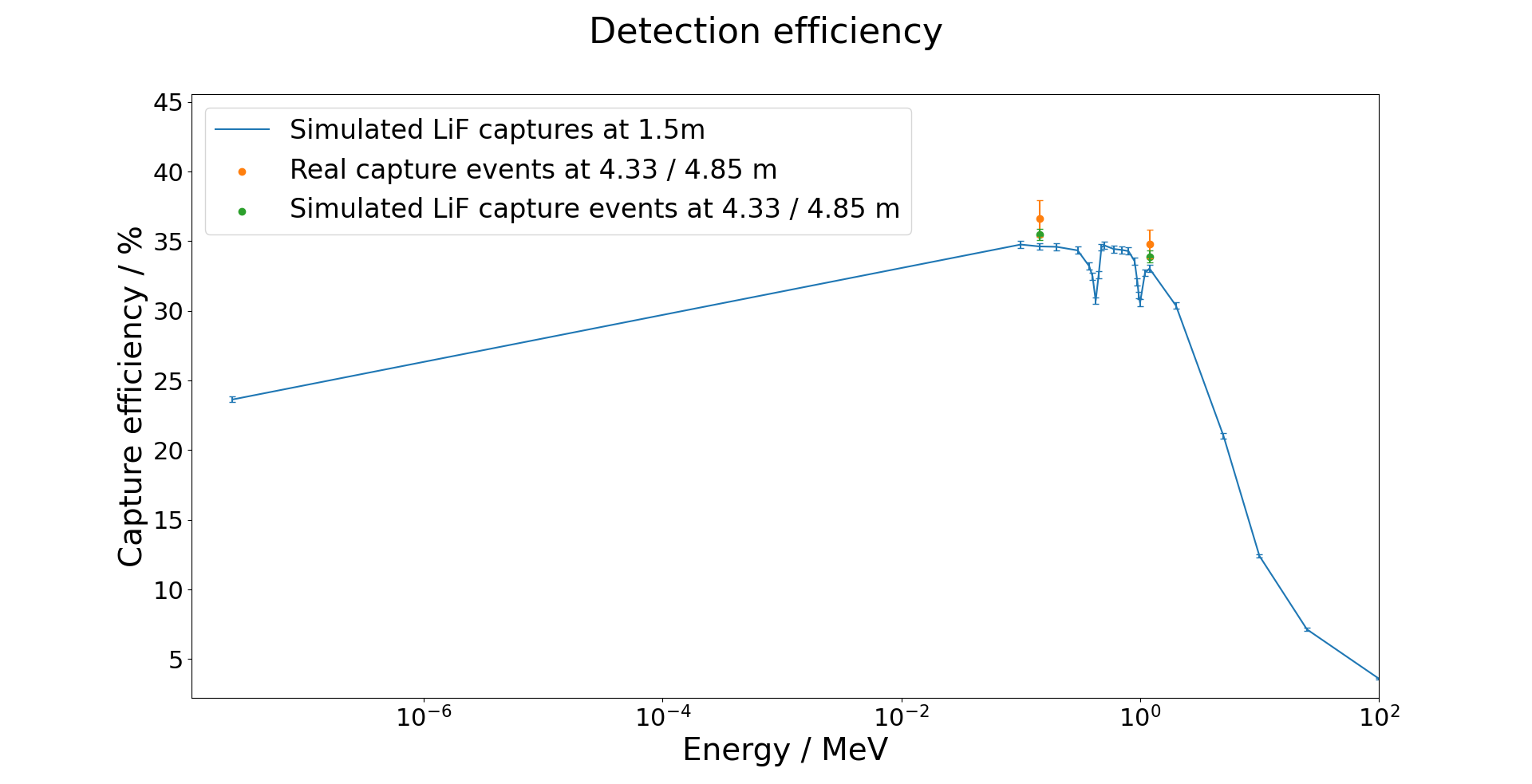Figure 10: \(^{6}\)Li neutron capture efficiency for simulated data and real data taken at NPL. The real data is consistent with the simulated data at the same distance within 1\(\sigma\).

After correcting the incident count calculation, the real and simulated efficiencies are consistent at the 1\(\sigma\) level. However, we now discover some peculiar dips in the capture efficiency, centred around ~425 keV and ~1 MeV. Additional energies have been sampled around these points to ensure that it is a physical effect, as opposed to incorrect processing of those data sets. The hypothesised cause of these decreases in efficiency was the presence of resonances in scattering cross sections in the detector case. The cross sections for materials in the detector case are shown in Figure 11. Specifically of note are the first two resonances in the oxygen cross section. When we overlay this cross section with the simulated capture efficiency curve, we find that the dips in the capture efficiency do indeed correspond exactly with these resonances in the oxygen scattering cross section. This can be seen in Figure 12. As a result we attribute these dips to increased scattering on the case, due to this oxygen scattering resonance.

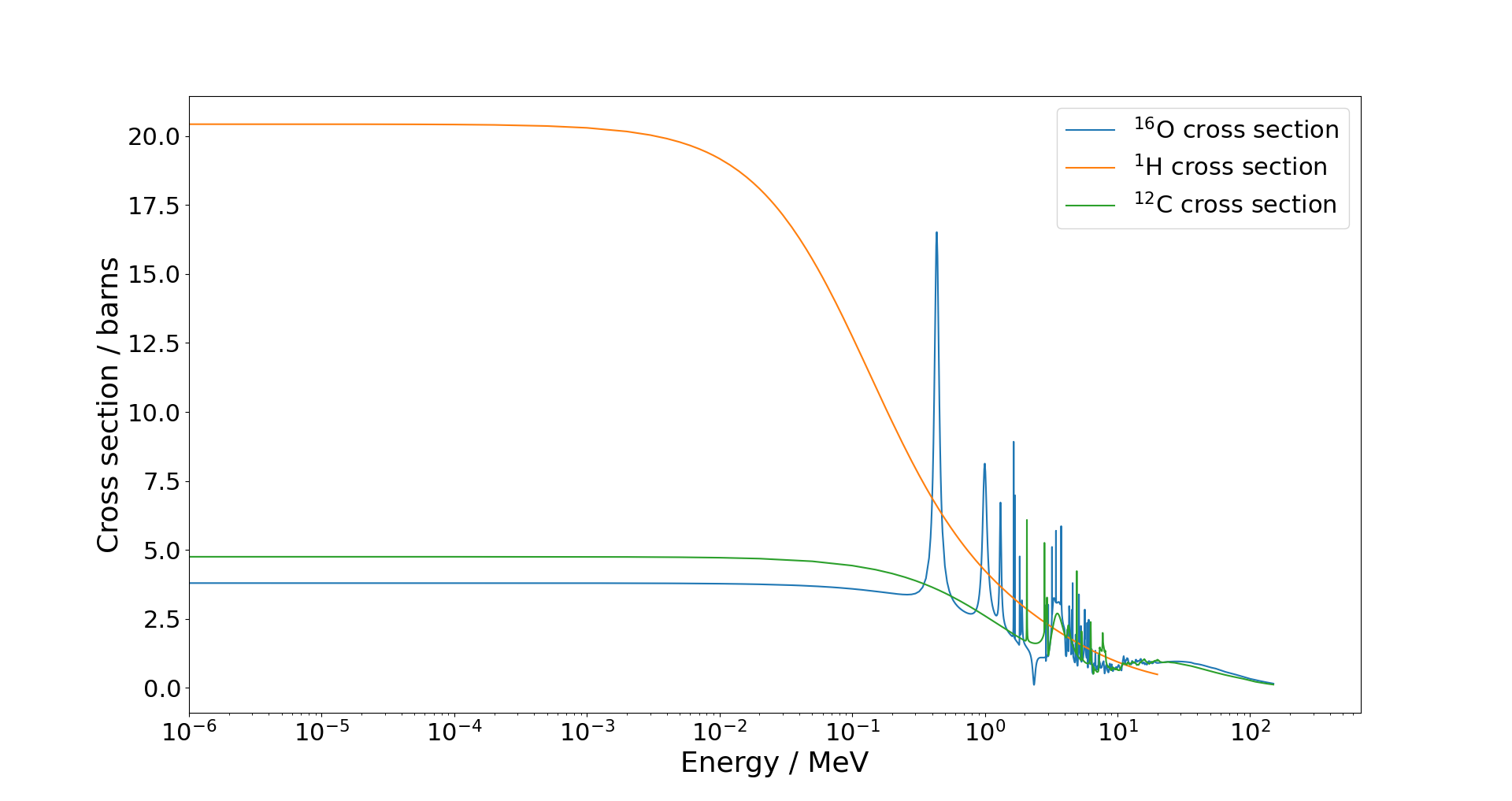Figure 11: Scattering cross sections for materials in the detector case. Hydrogen is the dominant scattering cross section until 1 MeV, but we also note resonances in the \(^{16}\)O cross section at ~400 keV and ~1 MeV that far exceed the hydrogen scattering cross section.

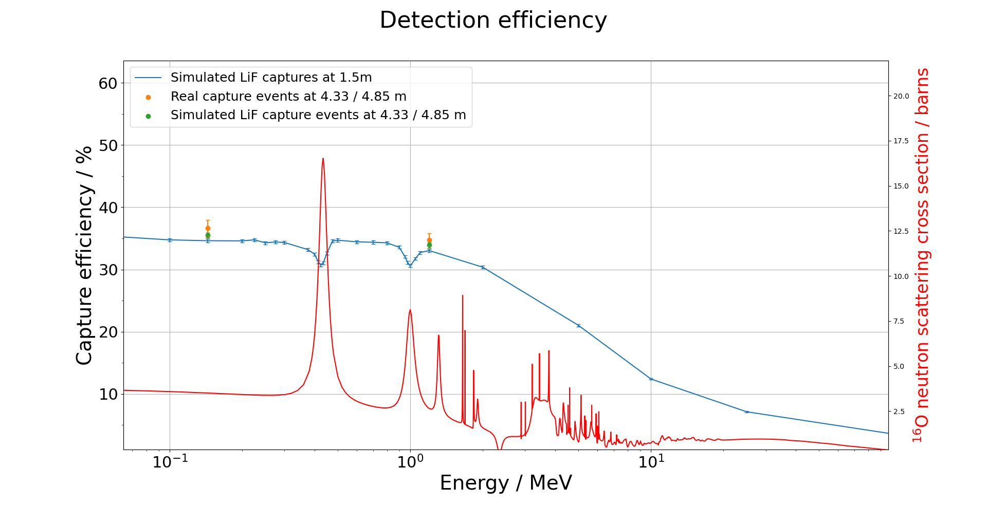Figure 12: Simulated capture efficiency compared with \(^{16}\)O cross section, as a function of energy. The dips in the capture efficiency correspond with resonances in the \(^{16}\)O cross section, so we attribute these dips to increased scattering on oxygen in the detector case.

Now that the simulated capture efficiency is well understood, it is important to consider how the angle of the detector to the source in the X-Y plane affects the the capture efficiency. It is expected that rotating the detector will have a significant effect on the capture efficiency due to the asymmetry of the placement of the LiF:ZnS screens, as discussed in Simulated LiF screen study. For multiples of 90\(^{\circ}\) we expect a separation of the efficiency curves between orientations with one of the screen-faces of the cube oriented towards the source, and those with the screen-faces oriented away from the source. The screens are facing towards the source at 0\(^{\circ}\) and 90\(^{\circ}\), and away from the source at 180\(^{\circ}\) and 270\(^{\circ}\). Similarly, for multiples of 45\(^{\circ}\), we anticipate a three groupings of efficiency curve based on the number of screen-faces oriented towards the source. These correspond to two (45:math:^{circ}), one (135:math:^{circ} and 315\(^{\circ}\), and zero (225:math:^{circ}) screen-faces oriented towards the source. Whilst preparing this data, a correction was made to the incident count once again, to properly account for neutrons incident on the corners of the case. The resulting updated simulated capture efficiency can be seen in Figure 13, and the simulated capture efficiencies at angles from 0\(^{\circ}\) to 315\(^{\circ}\) in increments of 45\(^{\circ}\) are shown in Figure 14.

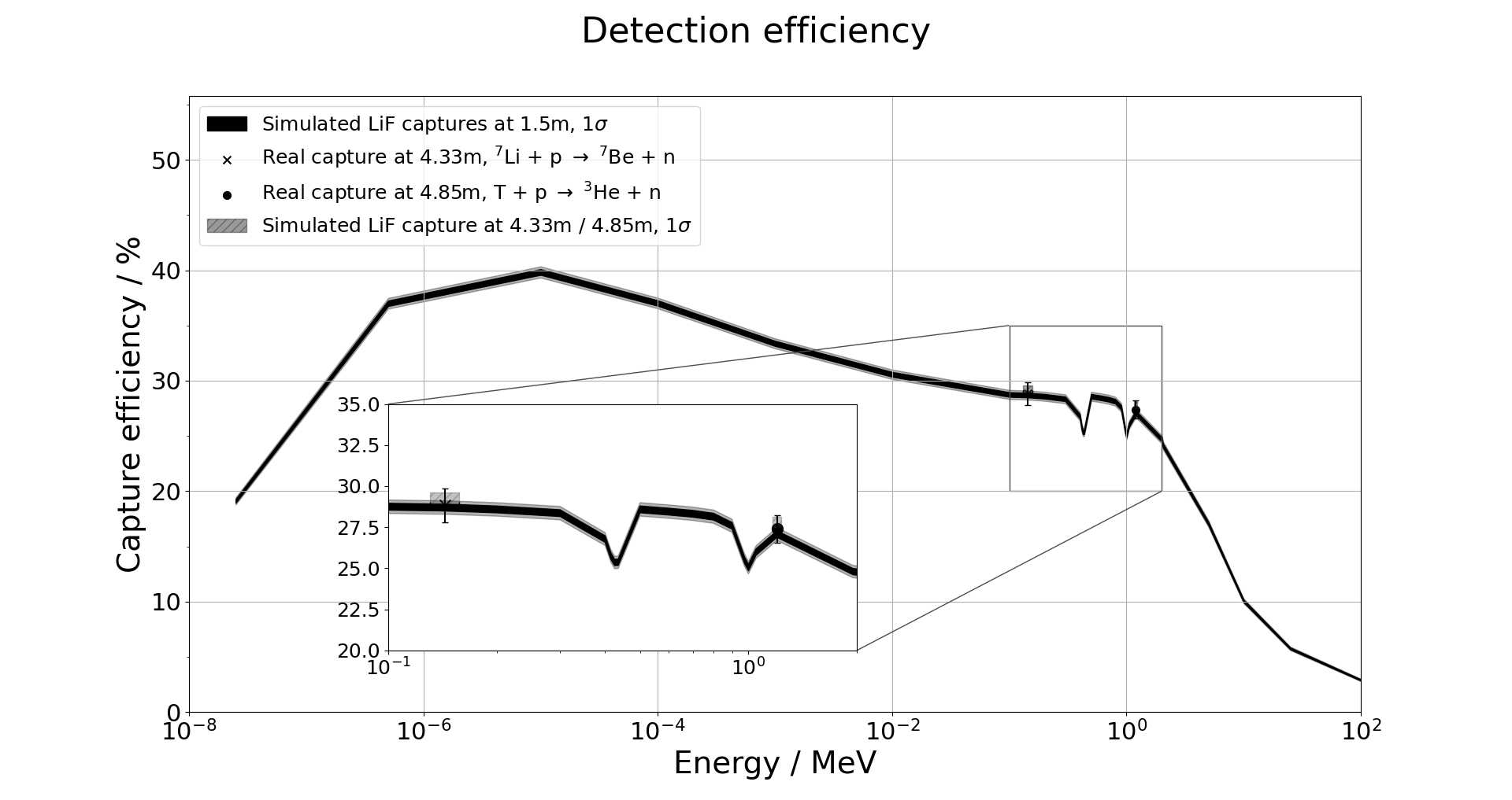Figure 13: The final simulated capture efficiency for neutrons incident on the Y = 3 face of the detector, compared with real data taken at NPL. The simulated and real data are in good agreement.

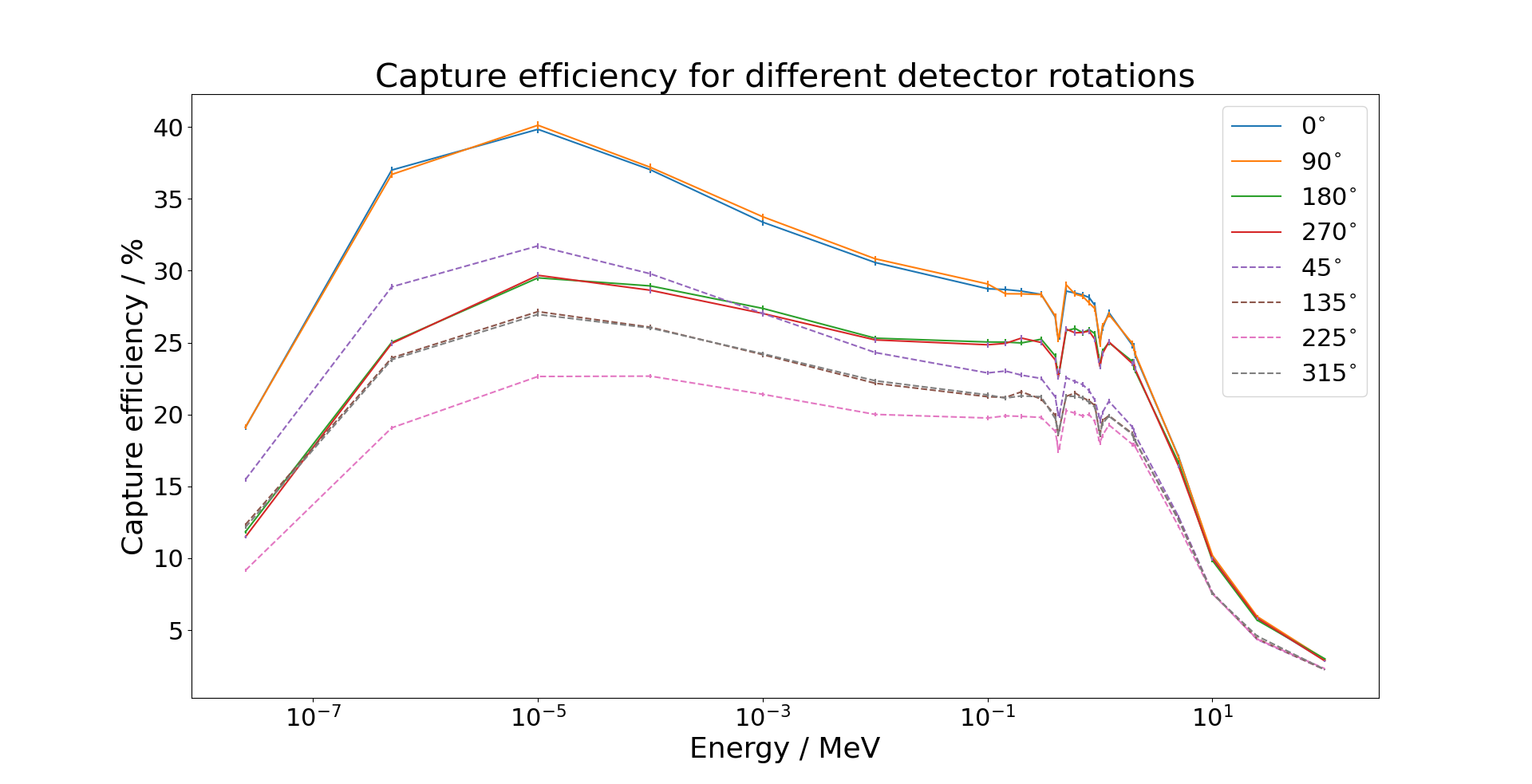Figure 14: The simulated capture efficiencies at 45\(^{\circ}\) increments. We note that the 45\(^{\circ}\) orientations generally have higher efficiency than the 180\(^{\circ}\) and 270\(^{\circ}\) orientations at low energies, as they have increased acceptance, but at higher energies efficiency is reduced as the volume of PVT each neutron passes through is on average lower for 45\(^{\circ}\) orientations.