Neural network for dose measurement

Introduction and motivation

In modern dosimetry, the gold standard of radiation dose measurement is effective dose. This quantity is defined as a sum over dose to each major organ in the human body, weighted by a set of tissue weighting factors that encode the average risk to health of a dose to that organ. This is a complex and difficult measurement to make, as many modern dosimeters are either optimised for field direction measurement or a fluence measurement. For example, for a Bonner sphere spectrometer, measuring effective dose is a time-consuming and computationally intensive process that requires careful measurement of the radiation field with varying size of polyethylene sphere and a complex unfolding algorithm to reconstruct the fluence, and this still lacks directional information about the field.

In contrast, the segmentation of nFacet 3D encodes both the direction and the energy of an incident neutron field. This can be visualised through the direction and intensity of attenuation of neutron count in the detector cubes. There are therefore two components to measuring the effective dose: reconstructing the fluence of the incident neutron field, and the direction of incidence of the neutrons. Here an artificial neural network (ANN) is applied for fluence reconstrunction, as once trained this is a fast method for reconstructing the fluence without need for a complex unfolding algorithm.

Training inputs

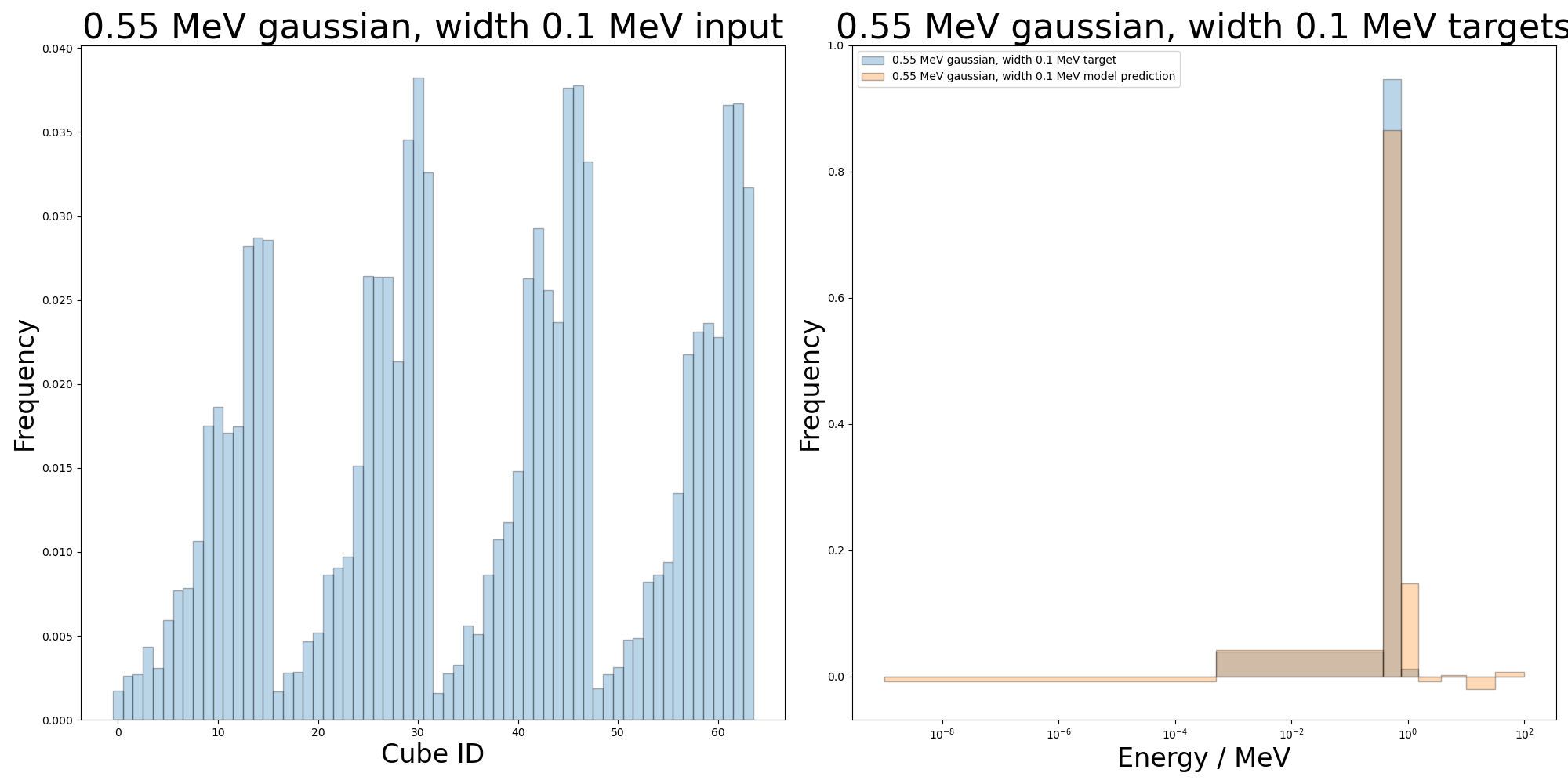
The neutron fluence is encoded in the distribution of counts across cubes in the detector, and as a result these counts are a natural choice for the neural network inputs. The data used for training the network was generated using a Geant4 simulation of the nFacet detector with the detector inside a Geant4 model of the low scattering facility at NPL. The geometry of this setup can be seen below.

MAKE SCHEMATICS (x-y, y-z)

The neutron spectrum of the source is specified at runtime, and each generated neutron is tracked until capture or reaching zero energy. The simulated detector registers counts for neutron capture on \(^{6}\)LiF:ZnS(Ag) and on PVT, and these two cases can be distinguished based on the particles remaining at the end of the track of a given neutron. The cube each hit occurs in is registered and saved, and individual neutrons can be grouped by the ID of the cube they capture in.

A unique ID number is assigned to each cube and the cube-level counts are flattened into a 1D array for input into the neural network. As the counts are normalised to sum to 1, the input given to the network is the fraction of counts in each cube.

There is also additional information encoded in the bulk response of the detector to an applied neutron field. By summing the counts in planes of cubes across the detector, we obtain 4 bins for each coordinate axis (X, Y and Z) which encode the attenuation length of the applied field in each of these directions. This can be appended to the cube-counts to produce a 76-length array as an input to the network. Each set of planes is normalised to 1 so that there is equal weighting between the cube counts and each set of plane counts.

As discussed in [put link to real vs sim here], there is good agreement between the results of the simulation and real-world data. As a result we use simulated data for training the neural network model, as it is easier and much cheaper to obtain than real datasets, whilst still describing the real situation well.

For this analysis, we assume a 3% uncertainty on the fractional counts in each cube or plane. This corresponds to a real measurement of approximately 64,000 neutrons which in turn gives an average of 1000 neutrons per detector cube, which results in a 3% Poisson error. By the central limit theorem, this is equivalent to a 3% Gaussian error as This is well motivated as this is size of dataset can be taken in ~10s of minutes at a source neutron rate of ~100 Hz, depending on the energy of the source. To augment the training dataset we take statistical resamples of each unique training data point, assuming the same 3% Gaussian uncertainty. This allows the network to learn the true distribution of cube counts for a given source, rather than learning the noise in the initial data points.

Training targets

The aim of this analysis is to reconstruct the fluence of the applied neutron field. In order to do this, the targets are taken to be a binned representation of the true fluence of each source. The specific energy binning scheme depends on the energy resolution of the detector, and we determine appropriate bin boundaries by looking for sources that the detector has sufficient resolution to distinguish. We calculate the absolute percentage difference of count in each cube between the two sources of interest, and any cubes with a difference greater than 3\(\sigma\) are deemed statistically distinguishable. We require that at least 75% of the cube counts are distinguishable in this way for two sources to be distinguishable. An example comparison of this kind is shown in Figure {NUMBER}.

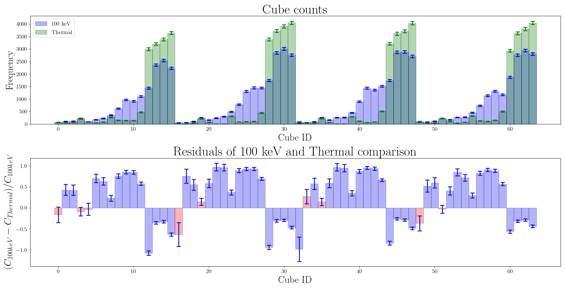
Figure 1: comparison between thermal and 100 keV neutron datasets. Top: the counts per cube in each dataset, along with the associated uncertainty. Total counts are normalised to 64,000 per dataset. Bottom: relative percentage difference between the two datasets. The red bins indicate cubes which are deemed to be statistically indistinguishable, as described above.

INCLUDE EXAMPLE PLOTS TO SHOW DISTINGUISHABLE SOURCES, REFERENCE APPENDIX TO SHOW ALL PLOTS?

Choice of training dataset

The training dataset comprised of several purely monoenergetic sources and some monoenergetic sources with a Gaussian spread, of various sizes. The full selection of sources used for training can be seen in the table below. The sources were selected such that each bin in the fluence targets would have the same number of training data points.

Type of source	Source energy	Source Gaussian spread
Pure monoenergetic	Thermal (0.025 eV)	N/A
	200, 400, 800 keV	N/A
	2, 5 MeV	N/A
Gaussian	1, 10, 25, 40 eV	10 eV
	50, 150, 250, 350, 450, 550, 650, 750, 850, 950 keV	100 keV
	1 MeV	200 keV
	1.4, 1.6 MeV	100 keV
	2.5, 3, 3.5, 4, 4.5 MeV	250 keV
	7, 9, 14, 18, 22, 26, 30 MeV	1 MeV
	40, 55, 70, 85, 100 MeV	5 MeV

Neural network architecture

The information for the network to learn is encoded in the distribution of neutron count across cubes in the detector. As a result, the first choice of input into the network consisted of 64 input neurons corresponding to the 64 cubes of the detector, whilst the output of the ANN was the binned fluence of the source in a total of 8 bins. The architecture of this model can be seen in Figure 1. When looking at various neural network models, we give them labels of the form “nnI_L1_L2_L3_…_O”, where I denotes the number of input neurons, Li denotes the number of neurons in hidden layer i, and O denotes the number of output neurons. The model discussed here is labelled as nn64_128_64_32_8.

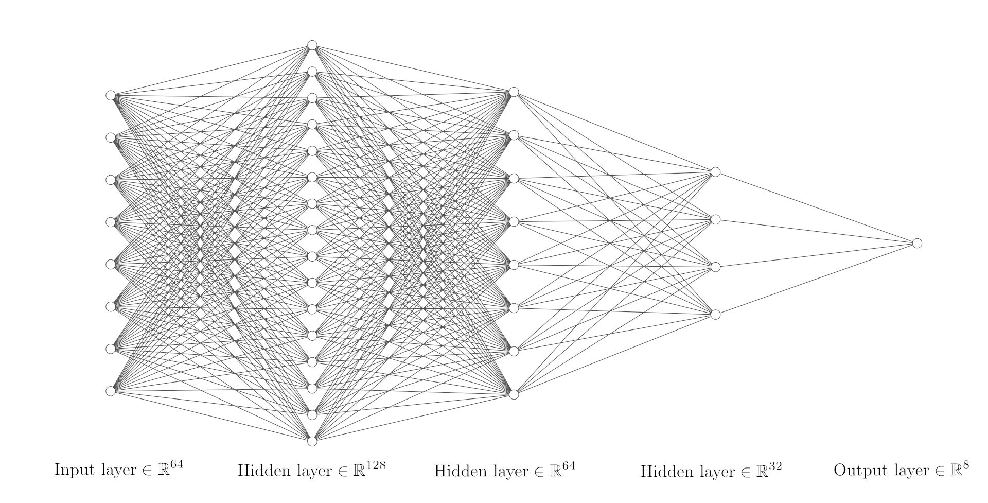Figure 2: graph of the nn64_128_64_32_8 model architecture. There are 64 input neurons corresponding to the 64 cubes of the detector, three hidden layers with ReLU activations, and 8 output neurons. In this diagram each node actually corresponds to 8 neurons, where all neurons are fully connected.

Additionally, summing the counts in planes of cubes provides additional information about the bulk response of the detector to the applied field and thus encodes more detailed information about the energy of the incident neutrons. This can be added to the inputs, adding 12 additional neurons corresponding to the four planes in the x, y and z directions. The number of neurons in hidden layers is also increased to fit the new data. We identify this model with the label nn76_152_76_38_8.

Analysis of error

In order to determine the effectiveness of the neural network, we must find the error on the effective dose predicted by the model, as this is the quantity of interest for this problem. As the model predicts a coarsely binned fluence, there is error not only from the model itself but also from the binning procedure when the continuous fluence of the source is coarsified into the energy bins used for the neural network targets. The dose conversion coefficients may vary significantly across the width of the bin but from the binned fluence the best estimate of the dose we can make is from the average dose coefficient in the bin, which can result in a significant error in the dose just from coarsifying the fluence. For dose calculations, the AP direction dose coefficients were used. For reference, here is the AP dose curve:

When calculating the dose from a binned fluence, the exact energies of the neutrons are not known and so instead dose must be calculated from an average dose per fluence for each bin. This average dose per fluence in each bin is found by integrating the dose coefficient curve over each bin and dividing by the bin width. Then, the total binned dose per fluence for each source is found by multiplying the counts in each bin for that source by the binned dose coefficients, and summing these products. This can be expressed as

\[D_{binned} = \sum_i c_i \frac{\int_i D(E) dE}{\Delta E_i},\]

where c_i denotes the count in bin i, D(E) denotes the dose coefficients as a function of energy, and \(\Delta E_i\) denotes the width in energy of bin i. For dose per fluence, these counts \(c_i\) should be normalised such that \(\sum_i c_i = 1\).

The true dose per fluence is found by integrating the product of the dose curve and the source distribution over the total energy range, given as

\[D_{true} = \int_0^\infty f(E) D(E) dE,\]

where f(E) is the true source distribution as a function of energy. This distribution is normalised such that \(\int_0^\infty f(E) dE = 1.\)

Finally, the relative dose per fluence error is expressed as \(\frac{D_{binned} - D_{true}}{D_{true}}\). This relative error resulting from the binning is shown in the table below.

Source	Relative binning error
Cf-252	1.2%
AmBe	-0.3%
AmLi	1.9%
144 keV	25.6%
1.2 MeV	-4.1%

Fluence binning scheme

TO BE ADDED

import os
import torch
from torch import nn
from torch.utils.data import DataLoader, random_split
import numpy as np
import pandas as pd

import matplotlib.pyplot as plt
import matplotlib.patches as mpatches
%matplotlib tk

import NNPytorchLightning as NNPL
from NNPytorchLightning import FluenceReconDataset, Resample


import warnings
from scipy.integrate import quad,IntegrationWarning
from scipy.interpolate import interp1d
from scipy.optimize import fminbound
warnings.simplefilter(action='ignore', category=IntegrationWarning)

Here loading trained models to compare the training and validation losses per model, and look at performance on unseen data. These models are as follows:

model_cubes: trained just on cube counts, with a batch size of 200 and 200 samples per data set, learning rate of 1e-3, for 500 epochs (for time)

model_cubes_profiles: trained on cube counts and profiles, with a batch size of 200 and 200 samples per data set, learning rate of 1e-3, for 500 epochs (for time)

coeffs = '/home/nr1315/Documents/Project/effective_dose_coeffs.h5'
energy_bins = '/home/nr1315/Documents/Project/MachineLearning/energy_bins.npy'

model_cubes = NNPL.LoadModel('/home/nr1315/Documents/Project/MachineLearning/lightning_logs/model_cubes_new_data/version_1/',torch.rand((1,1,64)),coeffs,energy_bins)

model_cubes_profiles = NNPL.LoadModel('/home/nr1315/Documents/Project/MachineLearning/lightning_logs/model_cubes_profiles_new_data/version_5/',torch.rand((1,1,76)),coeffs,energy_bins)

Also need to load the loss curves separately, due to the way they are from the logs.

model_cubes_tloss = pd.read_csv('/home/nr1315/Documents/Project/MachineLearning/LoggedParameters/run-model_cubes_new_data_version_1-tag-train_loss.csv')
model_cubes_vloss = pd.read_csv('/home/nr1315/Documents/Project/MachineLearning/LoggedParameters/run-model_cubes_new_data_version_1-tag-val_loss.csv')
model_cubes_dose_err = pd.read_csv('/home/nr1315/Documents/Project/MachineLearning/LoggedParameters/run-model_cubes_new_data_version_1-tag-dose_err_AP.csv')
model_cubes_epoch = pd.read_csv('/home/nr1315/Documents/Project/MachineLearning/LoggedParameters/run-model_cubes_new_data_version_1-tag-epoch.csv')

model_cubes_profiles_tloss = pd.read_csv('/home/nr1315/Documents/Project/MachineLearning/LoggedParameters/run-model_cubes_profiles_new_data_version_5-tag-train_loss.csv')
model_cubes_profiles_vloss = pd.read_csv('/home/nr1315/Documents/Project/MachineLearning/LoggedParameters/run-model_cubes_profiles_new_data_version_5-tag-val_loss.csv')
model_cubes_profiles_dose_err = pd.read_csv('/home/nr1315/Documents/Project/MachineLearning/LoggedParameters/run-model_cubes_profiles_new_data_version_5-tag-dose_err_AP.csv')
model_cubes_profiles_epoch = pd.read_csv('/home/nr1315/Documents/Project/MachineLearning/LoggedParameters/run-model_cubes_profiles_new_data_version_5-tag-epoch.csv')

We also define the directories from which to load the testing data, for convenience:

testing_data_dir = '/home/nr1315/Documents/Project/MachineLearning/TestingData/'

AmBe_counts = 'SimCubeCounts_AmBe_5_0-0-0-0-1-0_1500.npy'
AmLi_counts = 'SimCubeCounts_AmLi_5_0-0-0-0-1-0_1500.npy'
Cf_counts = 'SimCubeCounts_Cf252_6_0-0-0-0-1-0_1500.npy'

AmBe_target = 'SimEnergyBins_AmBe.npy'
AmLi_target = 'SimEnergyBins_AmLi.npy'
Cf_target = 'SimEnergyBins_Cf252.npy'

For each model in turn, we will look at the loss curves and prediction on AmBe, AmLi, and Cf-252.

Cubes only model, 500 epochs, 200 samples per dataset

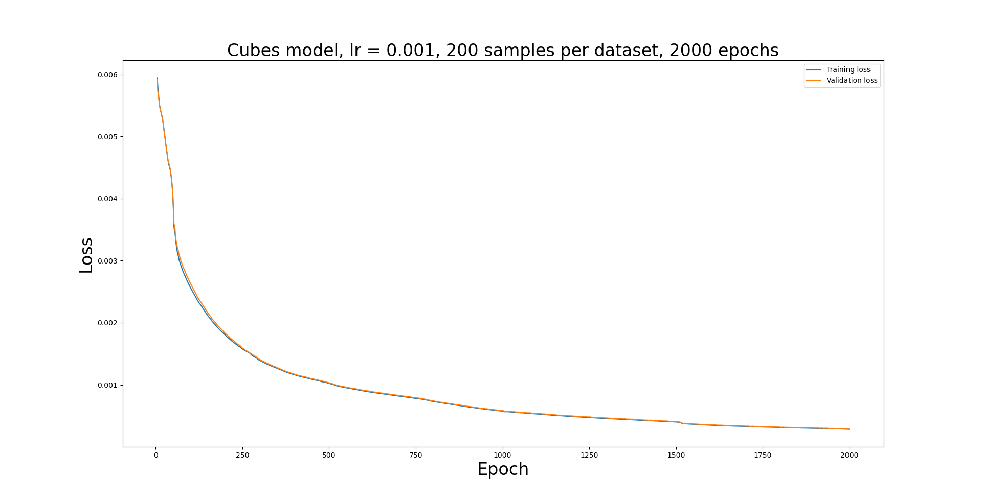
NNPL.PlotLosses([model_cubes_tloss,model_cubes_vloss],['Training loss','Validation loss'],'Cubes model, lr = 0.001, 200 samples per dataset',model_cubes_epoch)

/home/nr1315/miniconda3/envs/NewMLEnv/lib/python3.9/site-packages/scipy/interpolate/interpolate.py:623: RuntimeWarning: invalid value encountered in true_divide
  slope = (y_hi - y_lo) / (x_hi - x_lo)[:, None]
/home/nr1315/miniconda3/envs/NewMLEnv/lib/python3.9/site-packages/scipy/interpolate/interpolate.py:623: RuntimeWarning: invalid value encountered in true_divide
  slope = (y_hi - y_lo) / (x_hi - x_lo)[:, None]

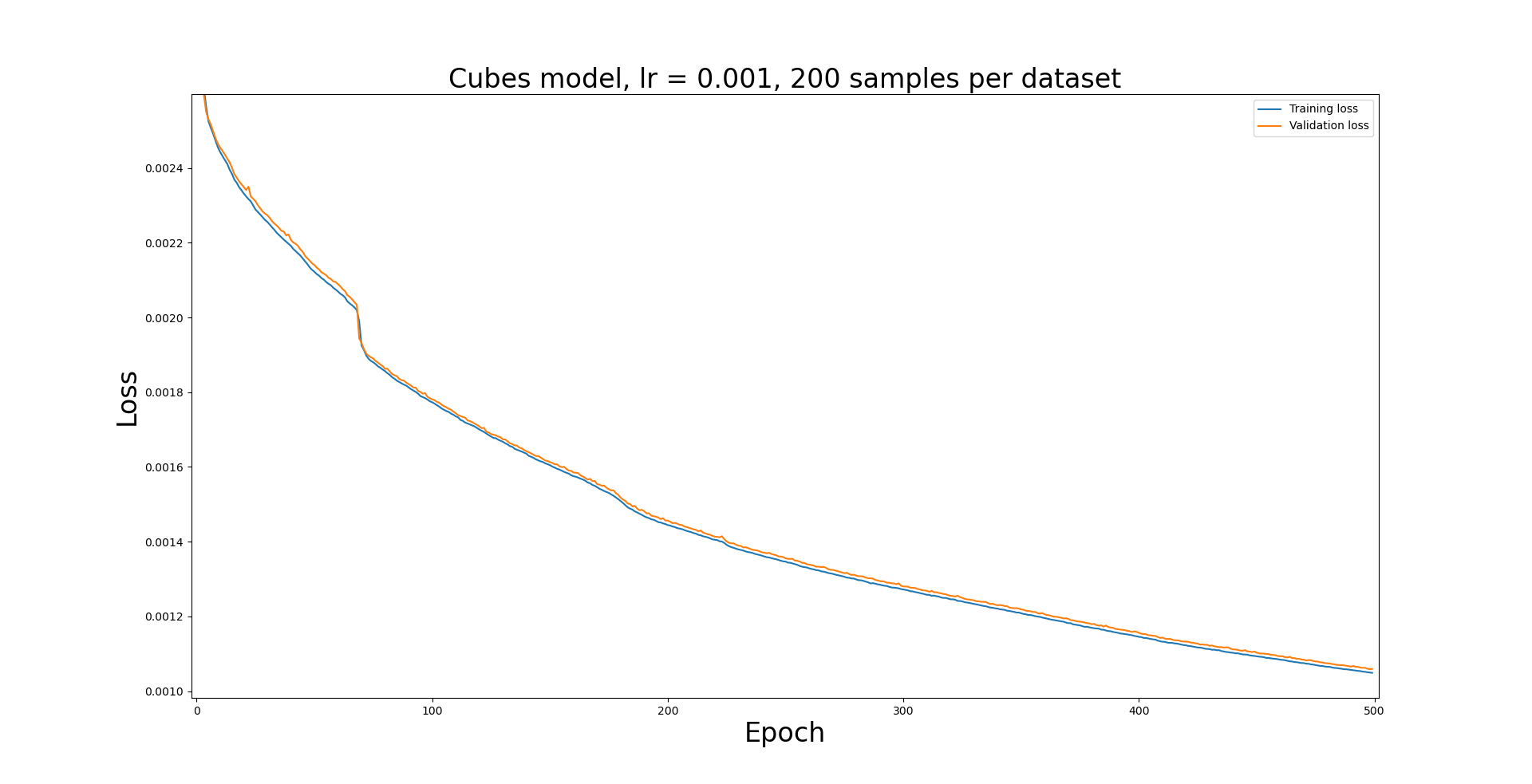
Here the model seems to be training well, although it does not appear to finish training after 500 epochs.

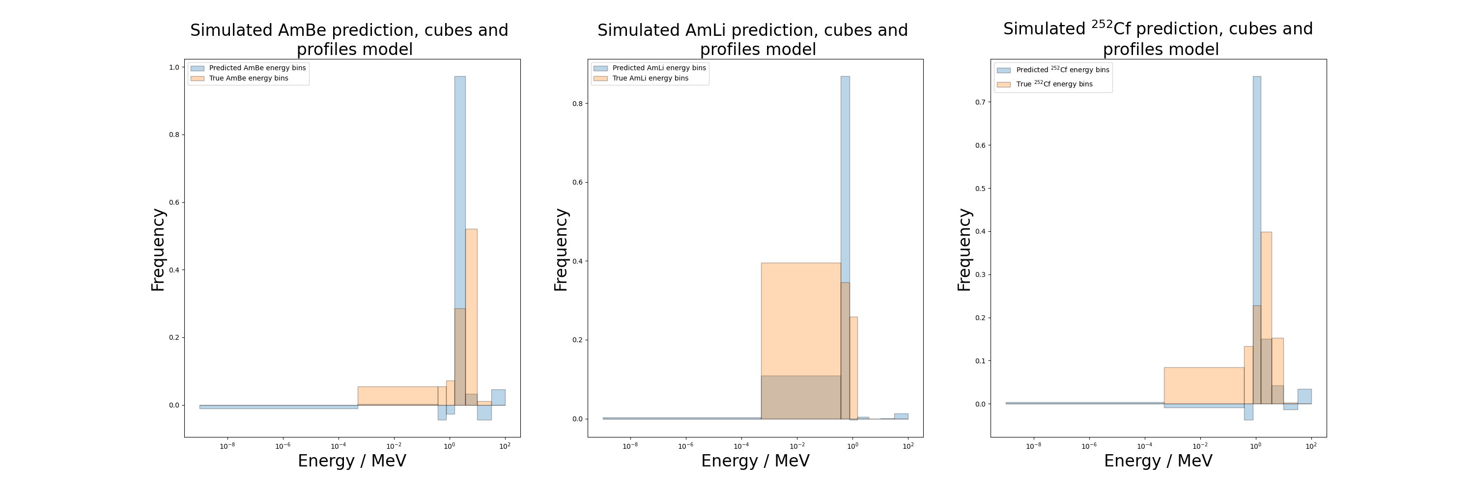
It is also informative to look at the quality of model prediction on unseen data, in this case AmLi, AmBe, and Cf252 sources. These can be seen below.

fig,ax = plt.subplots(1,3,figsize=(30,10))

loss_fn = nn.MSELoss()

AmBe_loss,AmBe_dose_err = NNPL.compare_pred_true(model_cubes,testing_data_dir+AmBe_counts,testing_data_dir+AmBe_target,'AmBe','cubes only model',ax[0],24,np.load(energy_bins),1,loss_fn,'AP')
AmLi_loss,AmLi_dose_err = NNPL.compare_pred_true(model_cubes,testing_data_dir+AmLi_counts,testing_data_dir+AmLi_target,'AmLi','cubes only model',ax[1],24,np.load(energy_bins),1,loss_fn,'AP')
Cf_loss,Cf_dose_err = NNPL.compare_pred_true(model_cubes,testing_data_dir+Cf_counts,testing_data_dir+Cf_target,r'$^{252}$Cf','cubes only model',ax[2],24,np.load(energy_bins),1,loss_fn,'AP')

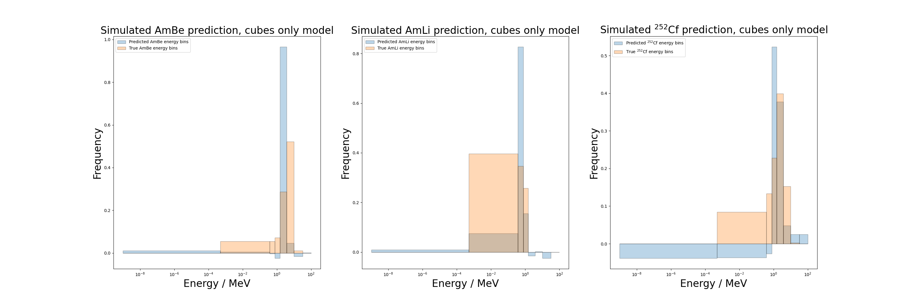
Whilst the model loss continues to decrease, the model still has poor performance on the unseen sources, predicting negative values in at least half the bins in all three cases. It generally seems to predict the greatest count in the region around the average energy of each source, i.e. above, below and at 1 MeV for AmBe, AmLi and Cf respectively, as previous iterations of the model did. One possible way to combat this may be to introduce more complex sources into the training set, such as linear combinations of existing monoenergetics, to help the network learn how to better reconstruct a more complicated fluence.

It is then informative to see the performance of the model on some of the validation data explicitly, as is shown below. The function used to plot this can be used to scroll through all of the training datasets.

cubes_dataloader = torch.load('/home/nr1315/Documents/Project/MachineLearning/lightning_logs/model_cubes_new_data/version_1/val_dloader.pt')
cubes_dataset,cubes_val_inds = cubes_dataloader.dataset.dataset,cubes_dataloader.dataset.indices

check = NNPL.CheckTrainData(model_cubes,cubes_dataset,np.load(energy_bins))

check.ViewTrainData()

The model has generally performed well at predicting the bins for this validation data point with some count in an incorrect bin, but of note is that it is still predicting negative values in several bins. In order to avoid this, it may prove useful to add a term to the loss function that penalises any negative bins in the model prediction.

A more thorough check of the validation data set for both this model and the following will be performed later.

Cubes and profiles model, 200 samples per dataset, learning rate 0.001

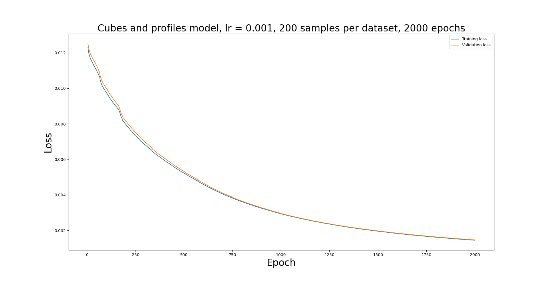
NNPL.PlotLosses([model_cubes_profiles_tloss,model_cubes_profiles_vloss],['Training loss','Validation loss'],'Cubes and profiles model, lr = 0.001, 200 samples per dataset',model_cubes_profiles_epoch)

/home/nr1315/miniconda3/envs/NewMLEnv/lib/python3.9/site-packages/scipy/interpolate/interpolate.py:623: RuntimeWarning: invalid value encountered in true_divide
  slope = (y_hi - y_lo) / (x_hi - x_lo)[:, None]
/home/nr1315/miniconda3/envs/NewMLEnv/lib/python3.9/site-packages/scipy/interpolate/interpolate.py:623: RuntimeWarning: invalid value encountered in true_divide
  slope = (y_hi - y_lo) / (x_hi - x_lo)[:, None]

Whilst both the training loss and validation loss do both decrease, it is worth noting that the validation loss here is lower than the training loss, which in turn implies that the model needs to train for longer in this configuration. This is intuitive, as the increased number of bins due to the profile counts will mean there are a greater number of weights for the model to optimize. Other improvements may be found from increasing the learning rate or adding some learning rate scheduling, but otherwise training for longer is realistically required.

It is also worthy of note that the loss is higher than for the cubes-only model, but this may be a factor of the incomplete training.

fig,ax = plt.subplots(1,3,figsize=(30,10))

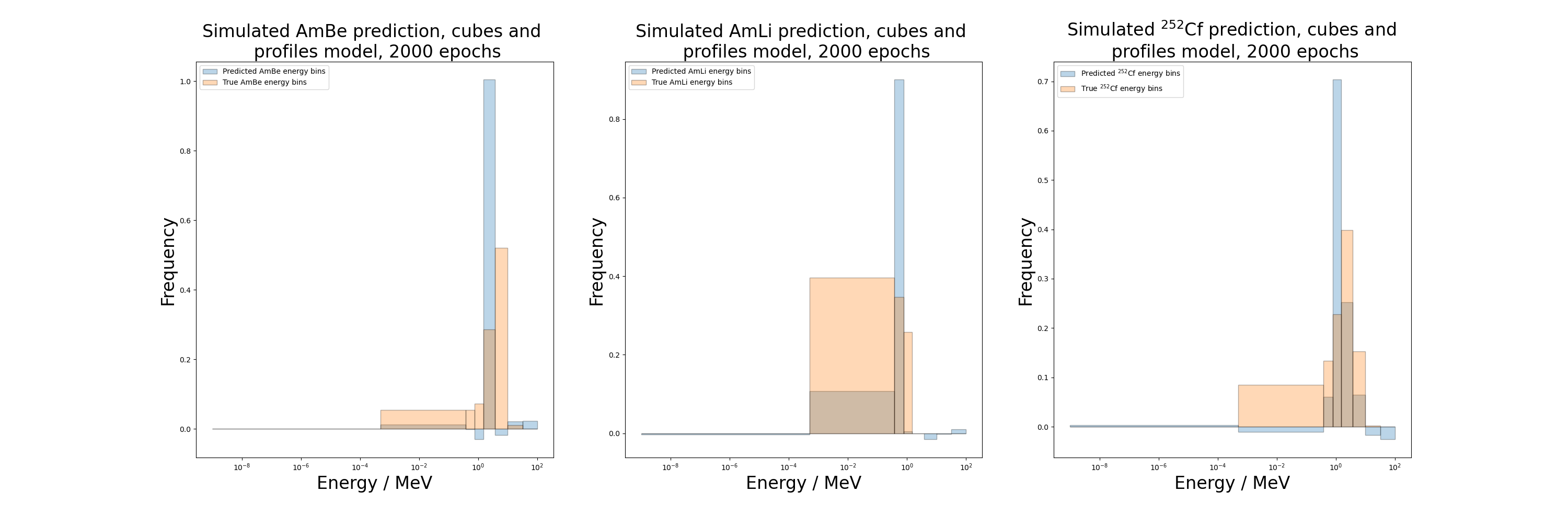
cp_AmBe_loss,cp_AmBe_dose_err = NNPL.compare_pred_true(model_cubes_profiles,testing_data_dir+'withProfiles/'+AmBe_counts,testing_data_dir+AmBe_target,'AmBe','cubes and \n profiles model',ax[0],24,np.load(energy_bins),1,loss_fn,'AP')
cp_AmLi_loss,cp_AmLi_dose_err = NNPL.compare_pred_true(model_cubes_profiles,testing_data_dir+'withProfiles/'+AmLi_counts,testing_data_dir+AmLi_target,'AmLi','cubes and \n profiles model',ax[1],24,np.load(energy_bins),1,loss_fn,'AP')
cp_Cf_loss,cp_Cf_dose_err = NNPL.compare_pred_true(model_cubes_profiles,testing_data_dir+'withProfiles/'+Cf_counts,testing_data_dir+Cf_target,r'$^{252}$Cf','cubes and \n profiles model',ax[2],24,np.load(energy_bins),1,loss_fn,'AP')

print("AmBe dose error: {}".format(100*cp_AmBe_dose_err))
print("AmLi dose error: {}".format(100*cp_AmLi_dose_err))
print("Cf dose error: {}".format(100*cp_Cf_dose_err))

AmBe dose error: 1.065460692649702
AmLi dose error: 3.1880135887862817
Cf dose error: 7.416363308539327

This model also performs poorly on the unseen data, although it has a lower loss than the cubes exclusive model. Most notably, this model predicts a large negative value in the first bin for all three sources, which further motivates introducing a penalty term to the loss to discourage any negative values in the model output.

Validation data set checking needs some more work before conclusions can be drawn.

cubes_profiles_dataloader = torch.load('/home/nr1315/Documents/Project/MachineLearning/lightning_logs/model_cubes_profiles_new_data/version_5/val_dloader.pt')
cubes_profiles_dataset,cubes_profiles_val_inds = cubes_profiles_dataloader.dataset.dataset,cubes_profiles_dataloader.dataset.indices

check = NNPL.CheckTrainData(model_cubes_profiles,cubes_profiles_dataset,np.load(energy_bins))

check.ViewTrainData()

After these results both models were trained again for 2000 epochs, as it appeared that neither model had fully trained in the 500 epochs here. These models and the monitoring quantities are loaded in here.

model_cubes_2000 = NNPL.LoadModel('/home/nr1315/Documents/Project/MachineLearning/lightning_logs/model_cubes_new_data/version_4/',torch.rand((1,1,64)),coeffs,energy_bins)

model_cubes_profiles_2000 = NNPL.LoadModel('/home/nr1315/Documents/Project/MachineLearning/lightning_logs/model_cubes_profiles_new_data/version_11/',torch.rand((1,1,76)),coeffs,energy_bins)

model_cubes_2000_tloss = pd.read_csv('/home/nr1315/Documents/Project/MachineLearning/LoggedParameters/run-model_cubes_new_data_version_4-tag-train_loss.csv')
model_cubes_2000_vloss = pd.read_csv('/home/nr1315/Documents/Project/MachineLearning/LoggedParameters/run-model_cubes_new_data_version_4-tag-val_loss.csv')
model_cubes_2000_dose_err = pd.read_csv('/home/nr1315/Documents/Project/MachineLearning/LoggedParameters/run-model_cubes_new_data_version_4-tag-dose_err_AP.csv')
model_cubes_2000_epoch = pd.read_csv('/home/nr1315/Documents/Project/MachineLearning/LoggedParameters/run-model_cubes_new_data_version_4-tag-epoch.csv')

model_cubes_profiles_2000_tloss = pd.read_csv('/home/nr1315/Documents/Project/MachineLearning/LoggedParameters/run-model_cubes_profiles_new_data_version_11-tag-train_loss.csv')
model_cubes_profiles_2000_vloss = pd.read_csv('/home/nr1315/Documents/Project/MachineLearning/LoggedParameters/run-model_cubes_profiles_new_data_version_11-tag-val_loss.csv')
model_cubes_profiles_2000_dose_err = pd.read_csv('/home/nr1315/Documents/Project/MachineLearning/LoggedParameters/run-model_cubes_profiles_new_data_version_11-tag-dose_err_AP.csv')

model_cubes_profiles_2000_epoch = pd.read_csv('/home/nr1315/Documents/Project/MachineLearning/LoggedParameters/run-model_cubes_profiles_new_data_version_11-tag-epoch.csv')

Cubes model, learning rate 0.001, 200 samples per dataset, trained for 2000 epochs

NNPL.PlotLosses([model_cubes_2000_tloss,model_cubes_2000_vloss],['Training loss','Validation loss'],'Cubes model, lr = 0.001, 200 samples per dataset, 2000 epochs',model_cubes_2000_epoch,log=False)

NNPL.PlotDoseError(model_cubes_2000_dose_err,'Cubes model, lr = 0.001, 200 samples per dataset, 2000 epochs, dose error',model_cubes_2000_epoch)

fig,ax = plt.subplots(1,3,figsize=(30,10))

loss_fn = nn.MSELoss()

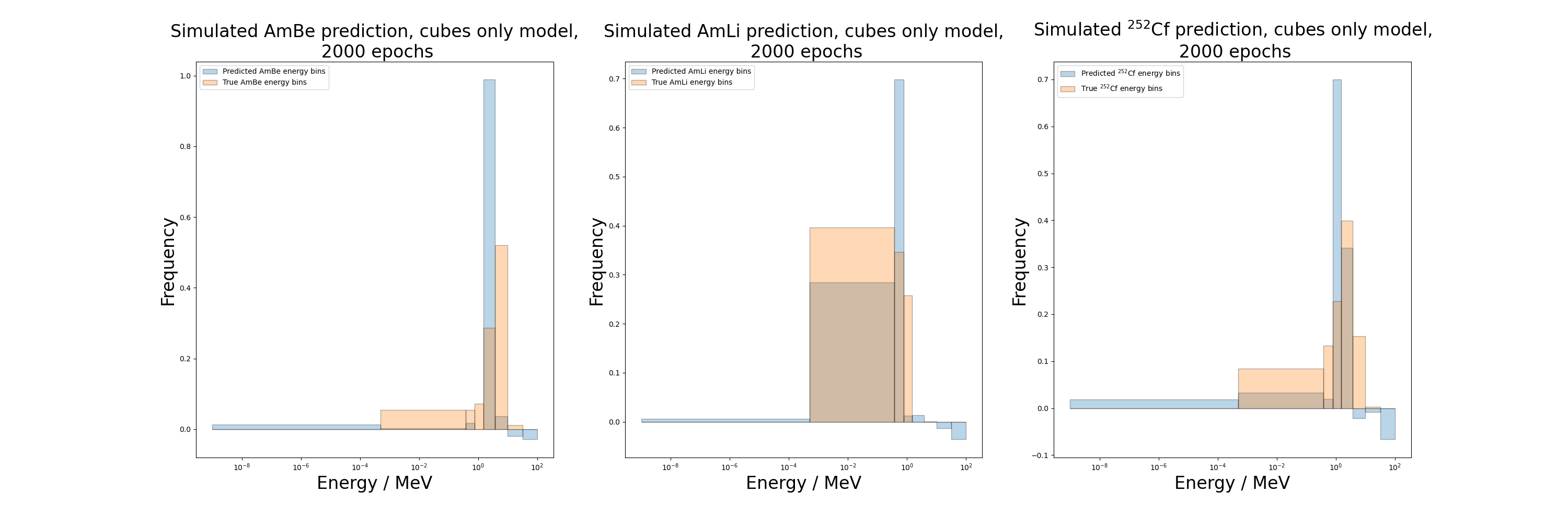
cubes_2000_AmBe_loss,cubes_2000_AmBe_dose_err = NNPL.compare_pred_true(model_cubes_2000,testing_data_dir+AmBe_counts,testing_data_dir+AmBe_target,'AmBe','cubes only model,\n 2000 epochs',ax[0],24,np.load(energy_bins),1,loss_fn,'AP')
cubes_2000_AmLi_loss,cubes_2000_AmLi_dose_err = NNPL.compare_pred_true(model_cubes_2000,testing_data_dir+AmLi_counts,testing_data_dir+AmLi_target,'AmLi','cubes only model,\n 2000 epochs',ax[1],24,np.load(energy_bins),1,loss_fn,'AP')
cubes_2000_Cf_loss,cubes_2000_Cf_dose_err = NNPL.compare_pred_true(model_cubes_2000,testing_data_dir+Cf_counts,testing_data_dir+Cf_target,r'$^{252}$Cf','cubes only model,\n 2000 epochs',ax[2],24,np.load(energy_bins),1,loss_fn,'AP')

print("AmBe loss: {}".format(cubes_2000_AmBe_loss))
print("AmLi loss: {}".format(cubes_2000_AmLi_loss))
print("Cf-252 loss: {}".format(cubes_2000_Cf_loss))

AmBe loss: 0.0924101173877716
AmLi loss: 0.02471756935119629
Cf-252 loss: 0.034533705562353134

print("AmBe {}".format(100*cubes_2000_AmBe_dose_err))
print("AmLi {}".format(100*cubes_2000_AmLi_dose_err))
print("Cf {}".format(100*cubes_2000_Cf_dose_err))

AmBe 1.2531776280353704
AmLi 17.97001801529823
Cf 5.568272436953861

Cubes and profiles model, learning rate 0.001, 200 samples per dataset, trained for 2000 epochs

NNPL.PlotLosses([model_cubes_profiles_2000_tloss,model_cubes_profiles_2000_vloss],['Training loss','Validation loss'],'Cubes and profiles model, lr = 0.001, 200 samples per dataset, 2000 epochs',model_cubes_profiles_2000_epoch,log=False)

NNPL.PlotDoseError(model_cubes_profiles_2000_dose_err,'Cubes and profiles model dose error',model_cubes_profiles_2000_epoch)

fig,ax=plt.subplots(1,3,figsize=(30,10))

cubes_profiles_2000_AmBe_loss,cp_2000_AmBe_dose_err = NNPL.compare_pred_true(model_cubes_profiles_2000,testing_data_dir+'withProfiles/'+AmBe_counts,testing_data_dir+AmBe_target,'AmBe','cubes and \n profiles model, 2000 epochs',ax[0],24,np.load(energy_bins),1,loss_fn,'AP')
cubes_profiles_2000_AmLi_loss,cp_2000_AmLi_dose_err = NNPL.compare_pred_true(model_cubes_profiles_2000,testing_data_dir+'withProfiles/'+AmLi_counts,testing_data_dir+AmLi_target,'AmLi','cubes and \n profiles model, 2000 epochs',ax[1],24,np.load(energy_bins),1,loss_fn,'AP')
cubes_profiles_2000_Cf_loss,cp_2000_Cf_dose_err = NNPL.compare_pred_true(model_cubes_profiles_2000,testing_data_dir+'withProfiles/'+Cf_counts,testing_data_dir+Cf_target,r'$^{252}$Cf','cubes and \n profiles model, 2000 epochs',ax[2],24,np.load(energy_bins),1,loss_fn,'AP')

print("AmBe loss: {}".format(cubes_profiles_2000_AmBe_loss))
print("AmLi loss: {}".format(cubes_profiles_2000_AmLi_loss))
print("Cf-252 loss: {}".format(cubes_profiles_2000_Cf_loss))

AmBe loss: 0.10277150571346283
AmLi loss: 0.05674799904227257
Cf-252 loss: 0.03377455845475197

print("AmBe: {}".format(cp_2000_AmBe_dose_err*100))
print("AmLi: {}".format(cp_2000_AmLi_dose_err*100))
print("Cf: {}".format(cp_2000_Cf_dose_err*100))

AmBe: 3.3541519263668786
AmLi: 1.2462487568431224
Cf: 0.891351256055962

Current results & future steps

Prediction on the test data is approximately equivalently bad for all of these models. All models seem to have learned to predict significant values in at most 2 or 3 bins, likely as the vase majority of the sources used for training only have counts in at most 3 bins. A way of tackling this would be to augment the training dataset with sources that are continuous across more bins than the existing data points, which could be accomplished in several ways:

• Generating additional training data with a greater spread in energy (e.g. larger Gaussian spread), such that individual data points cover more energy bins

• Implementing a transform to produce new data points composed of a linear combination of two or more existing data points

• Training on 1 or 2 of the test sources, to see if that improves prediction on the third (and on more complex sources in general)

Whilst the first approach is straightforward, it will add data points that peak around a particular bin and have a spread around that bin, rather than producing a more complex neutron spectrum that may have multiple peaks, although more complex distributions than a Gaussian could be used. It also would require generating a significant amount of additional training data, which is not storage efficient.

The second approach can in principle can teach the model more flexibility in how sources with a wide range of energies are encoded in the counts measured by the detector. This transformation would allow the model to learn an how an arbitrary fluence is encoded in the inputs, but in order to result in good prediction on real sources it may require some more careful logic on which sources are combined by the transformation, e.g. only taking those close in energy. However, following implementation of a rotation transform it may be informative to provide training data that is a composite of a high energy source on one side of the detector with a thermal source on the opposite side, to emulate a scenario with backscattered thermal neutrons.

Regarding the final approach eventually the model will be trained on all of these sources, but in the mean time training on one of these may be useful to test the ability of the model to learn a more continuous source on top of the monoenergetic sources it is already learning.

The model also can regularly predicit negative values in energy bins, when obviously this is not a physical result. In order to prevent this, I propose adding a term to the loss that penalises any bins with a negative value in the output. This could for example be done with a simple boolean check on each value in the output tensor, adding a factor k to the loss for each bin that has a negative value. This factor k could be tuned at initialisation of the loss function in order to tune how harshly the model penalises negative bins, and the ideal value of this parameter can be investigated.

A final point of note is how many epochs the model takes to train - even after 2000 epochs the training and validation losses are still decreasing, along with the average absolute percentage error on dose. This motivates revisiting the optimisation of the network, particularly looking at the learning rate or a learning rate scheduler, as well as the choice of optimisation algorithm.

We can also compare the model predictions to the true and binned doses for each respective testing source. In this analysis, the 144 keV and 1.2 MeV datasets used are real datasets taken at NPL in 2021, with the shadowcone measurement subtracted.

Source	Model	# of epochs	True dose per fluence / pSv cm\(^2\)	Binned dose per fluence / pSv cm\(^2\)	Relative binning error	Predicted dose per fluence / pSv cm\(^2\)	Prediction error vs target	Prediction error vs true
Cf\(^{252}\)	nn64_128_64_32_8	\(500\)	\(350.4\)	\(354.5^{+ 41.4}_{-59.1}\)	\(1.2\%\)	\(367.3^{+ 39.3}_{- 59.0}\)	\(3.6\%\)	\(4.8\%\)
		\(2000\)	\(350.4\)	\(354.5^{+ 41.4}_{-59.1}\)	\(1.2\%\)	\(333.3^{+ 49.8}_{- 71.4}\)	\(-6.0\%\)	\(-4.9\%\)
	nn76_152_76_38_8	\(500\)	\(350.4\)	\(354.5^{+ 41.4}_{-59.1}\)	\(1.2\%\)	\(194.6^{+ 26.4}_{- 35.6}\)	\(-45.1\%\)	\(-44.4\%\)
		\(2000\)	\(350.4\)	\(354.5^{+ 41.4}_{-59.1}\)	\(1.2\%\)	\(321.4^{+ 36.4}_{- 51.5}\)	\(-9.4\%\)	\(-8.3\%\)
AmBe	nn64_128_64_32_8	\(500\)	\(427.0\)	\(425.7^{+ 24.5}_{-41.8}\)	\(-0.3\%\)	\(426.9^{+ 40.3}_{- 65.5}\)	\(0.3\%\)	\(-0.02\%\)
		\(2000\)	\(427.0\)	\(425.7^{+ 24.5}_{-41.8}\)	\(-0.3\%\)	\(429.1_{- 68.8}^{+ 42.5}\)	\(0.8\%\)	\(0.5\%\)
	nn76_152_76_38_8	\(500\)	\(427.0\)	\(425.7^{+ 24.5}_{-41.8}\)	\(-0.3\%\)	\(207.7_{- 37.9}^{+ 27.9}\)	\(-51.2\%\)	\(-51.3\%\)
		\(2000\)	\(427.0\)	\(425.7^{+ 24.5}_{-41.8}\)	\(-0.3\%\)	\(315.0_{- 48.6}^{+ 34.0}\)	\(-26.0\%\)	\(-26.2\%\)
AmLi	nn64_128_64_32_8	\(500\)	\(175.4\)	\(178.7_{- 63.7}^{+ 56.4}\)	\(1.9\%\)	\(199.8_{- 62.4}^{+ 55.0}\)	\(11.8\%\)	\(13.9\%\)
		\(2000\)	\(175.4\)	\(178.7_{- 63.7}^{+ 56.4}\)	\(1.9\%\)	\(147.0_{- 60.5}^{+ 55.3}\)	\(-17.7\%\)	\(-16.2\%\)
	nn76_152_76_38_8	\(500\)	\(175.4\)	\(178.7_{- 63.7}^{+ 56.4}\)	\(1.9\%\)	\(165.4_{- 35.2}^{+ 27.5}\)	\(-7.4\%\)	\(-5.7\%\)
		\(2000\)	\(175.4\)	\(178.7_{- 63.7}^{+ 56.4}\)	\(1.9\%\)	\(210.3_{- 42.6}^{+ 33.5}\)	\(17.7\%\)	\(19.9\%\)
144 keV, shadowcone subtracted	nn64_128_64_32_8	\(500\)	\(58.4\)	\(73.3_{- 65.8}^{+ 64.3}\)	\(25.6\%\)	\(186.0_{- 71.3}^{+ 61.7}\)	\(154.0\%\)	\(218.8\%\)
		\(2000\)	\(58.4\)	\(73.3_{- 65.8}^{+ 64.3}\)	\(25.6\%\)	\(95.3_{- 48.3}^{+ 44.5}\)	\(30.0\%\)	\(63.3\%\)
	nn76_152_76_38_8	\(500\)	\(58.4\)	\(73.3_{- 65.8}^{+ 64.3}\)	\(25.6\%\)	\(161.9_{- 35}^{+ 27.6}\)	\(120.9\%\)	\(177.5\%\)
		\(2000\)	\(58.4\)	\(73.3_{- 65.8}^{+ 64.3}\)	\(25.6\%\)	\(198.5_{- 41.6}^{+ 33.3}\)	\(170.8\%\)	\(240.2\%\)
1.2 MeV, shadowcone subtracted	nn64_128_64_32_8	\(500\)	\(330.0\)	\(316.4_{- 66.8}^{+ 48.6}\)	\(-4.1\%\)	\(408.2_{- 69.2}^{+ 43.6}\)	\(29.0\%\)	\(23.7\%\)
		\(2000\)	\(330.0\)	\(316.4_{- 66.8}^{+ 48.6}\)	\(-4.1\%\)	\(381.1_{- 66.9}^{+ 44.3}\)	\(20.4\%\)	\(15.5\%\)
	nn76_152_76_38_8	\(500\)	\(330.0\)	\(316.4_{- 66.8}^{+ 48.6}\)	\(-4.1\%\)	\(203.5_{- 37.9}^{+ 28.1}\)	\(-35.7\%\)	\(-38.3\%\)
		\(2000\)	\(330.0\)	\(316.4_{- 66.8}^{+ 48.6}\)	\(-4.1\%\)	\(320.7_{- 50.6}^{+ 35.5}\)	\(1.4\%\)	\(-2.8\%\)

There are a few points of note from these results:

• In general, the error from the binning procedure is higher for the monoenergetic sources than the continuous sources. This is because the dose contribution from a given bin for a continuous source will be from a range of energies across that bin as opposed to from a single energy within the bin. As a result the continuous distribution across the bin effectively averages out the dose more than the monoenergetic source, thus meaning that the average dose coefficient used to calculate the binned dose is a closer match to the true dose.

• The relative error between the predicted dose and the true dose decreases as a function of energy for the models with only cubes included, whilst for the models including profiles it underestimates the error more at higher energies. This can be seen in more detail in the plot below.

MORE TO ADD

Working to be neatened

————————————————————————————————————————————————————–

def PrepDoseBounds(coeffs,bins,d):
    dose_curve = interp1d(coeffs['Energy / MeV'],coeffs[d])

    avg_dpf,max_dpf,min_dpf = [],[],[]
    for i in range(len(bins)-1):
        avg_dpf.append(quad(dose_curve,bins[i],bins[i+1],limit=200)[0])
        max_dpf.append(dose_curve(fminbound(lambda x : -1*dose_curve(x),bins[i],bins[i+1])))
        min_dpf.append(dose_curve(fminbound(dose_curve,bins[i],bins[i+1])))
    avg_dpf = np.array(avg_dpf)/np.diff(bins)
    max_dpf = np.array(max_dpf)
    min_dpf = np.array(min_dpf)

    return np.vstack([min_dpf,avg_dpf,max_dpf])

def UpperLowerBounds(coeffs,bins,d,bin_counts):
    dose_bounds = PrepDoseBounds(coeffs,bins,d)
    source_dose_bounds = (bin_counts*dose_bounds).sum(axis=1)
    return source_dose_bounds

UpperLowerBounds(dose_coeffs,bins,'AP',models[0](torch.from_numpy(inputs[0][0]/inputs[0][0].sum()).to(torch.float)).detach().numpy())

array([343.95263369, 409.77910069, 453.5938381 ])

def LoadRealCubes(dfile,sdc,profile):
    real_cubes,total_count,real_time = NNPL.PrepareRealInput(dfile,profile)

    if sdc is not None:
        sdc_cubes,sdc_count,sdc_time = NNPL.PrepareRealInput(sdc,profile)

        sub_cubes = (total_count*real_cubes/real_time - sdc_count*sdc_cubes/sdc_time)*min(real_time,sdc_time)
        sub_cubes = sub_cubes/sub_cubes.sum()
    else:
        sub_cubes = real_cubes/real_cubes.sum()

    return sub_cubes.flatten()

def CalcTrueDose(source_dist,d,coeffs):
    dose_curve = interp1d(coeffs['Energy / MeV'],coeffs[d])
    if callable(source_dist):
        true_dose = quad(lambda x:source_dist(x)*dose_curve(x),0,np.inf,limit=200)[0]
    else:
        true_dose = dose_curve(source_dist)
    return true_dose

Cf,Cf_bounds = NNPL.PrepareYieldDist('/home/nr1315/Documents/Project/MachineLearning/Cf252Yield.npy')
AmBe,AmBe_bounds = NNPL.PrepareYieldDist('/home/nr1315/Documents/Project/MachineLearning/AmBeYield.npy')
AmLi,AmLi_bounds = NNPL.PrepareYieldDist('/home/nr1315/Documents/Project/MachineLearning/AmLiYield.npy')

monos_144_cubes = LoadRealCubes('/home/nr1315/Documents/Project/NPL_2021/vdg_1um_Li7target19A_433cm_0deg.h5','/home/nr1315/Documents/Project/NPL_2021/vdg_1um_Li7target19A_433cm_0deg_shadowcone.h5',False)
monos_1_2_cubes = LoadRealCubes('/home/nr1315/Documents/Project/NPL_2021/vdg_1um_1_2_MeV_target3_2.h5','/home/nr1315/Documents/Project/NPL_2021/vdg_1um_1_2_MeV_target3_shadowcone.h5',False)
monos_144_profiles = LoadRealCubes('/home/nr1315/Documents/Project/NPL_2021/vdg_1um_Li7target19A_433cm_0deg.h5','/home/nr1315/Documents/Project/NPL_2021/vdg_1um_Li7target19A_433cm_0deg_shadowcone.h5',True)
monos_1_2_profiles = LoadRealCubes('/home/nr1315/Documents/Project/NPL_2021/vdg_1um_1_2_MeV_target3_2.h5','/home/nr1315/Documents/Project/NPL_2021/vdg_1um_1_2_MeV_target3_shadowcone.h5',True)

names = ['nn64_128_64_32_8, 500 epochs','nn76_152_76_38_8, 500 epochs','nn64_128_64_32_8, 2000 epochs','nn76_152_76_38_8, 2000 epochs']



bins = np.load(energy_bins)
dose_coeffs = pd.read_hdf(coeffs)

---------------------------------------------------------------------------
NameError                                 Traceback (most recent call last)
/tmp/ipykernel_29268/3173995836.py in <module>
      3 AmLi,AmLi_bounds = NNPL.PrepareYieldDist('/home/nr1315/Documents/Project/MachineLearning/AmLiYield.npy')
      4
----> 5 monos_144_cubes = LoadRealCubes('/home/nr1315/Documents/Project/NPL_2021/vdg_1um_Li7target19A_433cm_0deg.h5','/home/nr1315/Documents/Project/NPL_2021/vdg_1um_Li7target19A_433cm_0deg_shadowcone.h5',False)
      6 monos_1_2_cubes = LoadRealCubes('/home/nr1315/Documents/Project/NPL_2021/vdg_1um_1_2_MeV_target3_2.h5','/home/nr1315/Documents/Project/NPL_2021/vdg_1um_1_2_MeV_target3_shadowcone.h5',False)
      7 monos_144_profiles = LoadRealCubes('/home/nr1315/Documents/Project/NPL_2021/vdg_1um_Li7target19A_433cm_0deg.h5','/home/nr1315/Documents/Project/NPL_2021/vdg_1um_Li7target19A_433cm_0deg_shadowcone.h5',True)

NameError: name 'LoadRealCubes' is not defined

labels = ['144 keV','AmLi','1.2 MeV','Cf','AmBe']
models = [model_cubes,model_cubes_profiles,model_cubes_2000,model_cubes_profiles_2000]

source_dists = [0.144,AmLi,1.2,Cf,AmBe]
targets = [np.histogram(144e-3,bins=bins)[0],AmLi_bins,np.histogram(1.2,bins=bins)[0],Cf_bins,AmBe_bins]
inputs = [[monos_144_cubes,AmLi_cubes,monos_1_2_cubes,Cf_cubes,AmBe_cubes],
          [monos_144_profiles,AmLi_profiles,monos_1_2_profiles,Cf_profiles,AmBe_profiles]]
Cf_b,AmBe_b,AmLi_b,mono_144_b,mono_1_2_b = {},{},{},{},{}
dicts = [mono_144_b,AmLi_b,mono_1_2_b,Cf_b,AmBe_b]
for i in range(5):
        for j in range(4):
            true_dose = CalcTrueDose(source_dists[i],'AP',dose_coeffs)
            binned_dose = UpperLowerBounds(dose_coeffs,bins,'AP',targets[i]/targets[i].sum())
            pred_dose = UpperLowerBounds(dose_coeffs,bins,'AP',models[j](torch.from_numpy(inputs[j%2][i]/inputs[j%2][i].sum()).to(torch.float)).detach().numpy())
            dicts[i][names[j]] = {'true':true_dose,'binned':binned_dose,'pred':pred_dose}

energies = [0.144,0.553,1.2,2.176,4.211]
colors = {names[0]:'blue',names[1]:'green',names[2]:'red',names[3]:'orange'}
mins,maxs = [],[]
for name in names:
    vals,ubs,lbs = [],[],[]
    for d in dicts:
        vals.append((d[name]['pred'][1] - d[name]['true'])/d[name]['true'])
        ubs.append((d[name]['pred'][2] - d[name]['true'])/d[name]['true'])
        lbs.append((d[name]['pred'][0] - d[name]['true'])/d[name]['true'])
    plt.plot(energies,100*np.array(vals),label=name,color=colors[name],alpha=0.6)
    mins.append(min(vals))
    maxs.append(max(vals))
    #plt.errorbar(energies,vals,yerr = [lbs,ubs],capsize=10,fmt='none',color=colors[name],alpha=0.6)
plt.legend(fontsize=16)
plt.xlabel('Energy / MeV',fontsize=18)
plt.ylabel('Relative error / %',fontsize=18)
plt.title('Error on prediction of true dose for test data',fontsize=24)
plt.xticks(fontsize=16)
plt.yticks(fontsize=16)
plt.grid()
plt.ylim(100*(min(mins) - 0.1),100*(max(maxs) + 0.1))
plt.xlim(0,4.5)

plt.plot(np.repeat(0.553,10),np.linspace(100*(min(mins)-0.1),100*(max(maxs)+0.1),10),color='black',linestyle='--',lw=1)
plt.plot(np.repeat(2.176,10),np.linspace(100*(min(mins)-0.1),100*(max(maxs)+0.1),10),color='black',linestyle='--',lw=1)
plt.plot(np.repeat(4.211,10),np.linspace(100*(min(mins)-0.1),100*(max(maxs)+0.1),10),color='black',linestyle='--',lw=1)

plt.plot(np.linspace(0,4.5,10),np.repeat(0,10),color='black',lw=1)

#plt.text(0.553+0.01,160,'AmLi\navg E',fontsize=16)
plt.text(0.553+0.01,160,r'$\langle E_{AmLi} \rangle$',fontsize=16)
plt.text(2.176 + 0.01,160,r'$\langle E_{^{252}Cf} \rangle$',fontsize=16)
plt.text(4.211 + 0.01,160,r'$\langle E_{AmBe} \rangle$',fontsize=16)

Text(4.221, 160, '$\\langle E_{AmBe} \\rangle$')

100*(min(mins) - 0.1)

-61.36319401179273

np.linspace(100*(min(mins) - 0.1),100*(max(maxs) + 0.1),10)

array([-61.36319401, -26.74771054,   7.86777293,  42.48325641,
        77.09873988, 111.71422335, 146.32970682, 180.9451903 ,
       215.56067377, 250.17615724])

np.diff(((models[0](torch.from_numpy(inputs[0][0]/inputs[0][0].sum()).to(torch.float)).detach().numpy())*PrepDoseBounds(dose_coeffs,bins,'AP')).sum(axis=1))

array([59.00984482, 39.2775272 ])

dicts[0]

{'nn64_128_64_32_8': ((59.13374163451289, 41.37319290883062),
  (65.82646700401324, 43.814737411850274)),
 'nn76_152_76_38_8': ((59.13374163451289, 41.37319290883062),
  (83.21004446166847, 61.56899967260864)),
 'nn64_128_64_32_8_2000': ((59.13374163451289, 41.37319290883062),
  (70.26762644020357, 49.02129856247541)),
 'nn76_152_76_38_8_2000': ((59.13374163451289, 41.37319290883062),
  (70.64399666877745, 49.85281107023491))}

UpperLowerBounds(dose_coeffs,bins,'AP',Cf_bins)

(59.13374163451289, 41.37319290883062)

cfd = (PrepDoseBounds(dose_coeffs,bins,'AP')*Cf_bins/Cf_bins.sum()).sum(axis=1)
cfd[1] - cfd[0],cfd[2]-cfd[1]

(59.13374163451289, 41.37319290883062)

model_cubes(torch.from_numpy(Cf_cubes/Cf_cubes.sum()).to(torch.float)).detach().numpy()

array([-0.03849331, -0.03727394, -0.02635773,  0.52332836,  0.37729588,
        0.04819015,  0.02464751,  0.02510862], dtype=float32)

(PrepDoseBounds(dose_coeffs,bins,'AP')*model_cubes(torch.from_numpy(Cf_cubes/Cf_cubes.sum()).to(torch.float)).detach().numpy()).sum(axis=1)

array([308.33481773, 367.34466255, 406.62218975])

import numpy as np
import pandas as pd
from scipy.interpolate import interp1d

dose_coeffs = pd.read_hdf(coeffs)
bins = np.load(energy_bins)

ap_dose_curve = interp1d(dose_coeffs['Energy / MeV'],dose_coeffs['AP'])

---------------------------------------------------------------------------
NameError                                 Traceback (most recent call last)
/tmp/ipykernel_19910/3864481691.py in <module>
----> 1 dose_coeffs = pd.read_hdf(coeffs)
      2 bins = np.load(energy_bins)
      3
      4 ap_dose_curve = interp1d(dose_coeffs['Energy / MeV'],dose_coeffs['AP'])

NameError: name 'coeffs' is not defined

integral_bin_dose = []
maxima_energy,minima_energy = [],[]
for i in range(len(bins)-1):
    integral_bin_dose.append(quad(ap_dose_curve,bins[i],bins[i+1],limit=200)[0])
    maxima_energy.append(fminbound(lambda x : -1*ap_dose_curve(x),bins[i],bins[i+1]))
    minima_energy.append(fminbound(ap_dose_curve,bins[i],bins[i+1]))
integral_bin_dose = np.array(integral_bin_dose)/np.diff(bins)
maxima_energy = np.array(maxima_energy)
minima_energy = np.array(minima_energy)

min_dpf = ap_dose_curve(minima_energy)
max_dpf = ap_dose_curve(maxima_energy)
avg_dpf = integral_bin_dose

dose_per_fluence_bins = np.vstack([min_dpf,avg_dpf,max_dpf])

(dose_per_fluence_bins[1] - dose_per_fluence_bins[0])/dose_per_fluence_bins[0]

array([0.01930433, 8.7238059 , 0.42822664, 0.26749172, 0.18846897,
       0.04087018, 0.05467647, 0.05697613])

(dose_per_fluence_bins[1] - dose_per_fluence_bins[2])/dose_per_fluence_bins[2]

array([-0.01905808, -0.46725902, -0.21256423, -0.13315322, -0.09010639,
       -0.00753   , -0.04868181, -0.0578616 ])

cf_bins = np.load('/home/nr1315/Documents/Project/MachineLearning/TestingData/SimEnergyBins_Cf252.npy')

cf_bins = cf_bins/cf_bins.sum()

cf_avg_dpf = cf_bins*avg_dpf
cf_max_dpf = cf_bins*max_dpf
cf_min_dpf = cf_bins*min_dpf

cf_avg_dpf.sum()

354.5143061942601

cf_max_dpf.sum()

395.8874991030907

cf_min_dpf.sum()

295.3805645597472

real_cubes_144,total_count_144,time_144 = NNPL.PrepareRealInput('/home/nr1315/Documents/Project/NPL_2021/vdg_1um_Li7target19A_433cm_0deg.h5')
sdc_cubes_144,sdc_count_144,sdc_time_144 = NNPL.PrepareRealInput('/home/nr1315/Documents/Project/NPL_2021/vdg_1um_Li7target19A_433cm_0deg_shadowcone.h5')

true_dose_144,true_count_144,true_count_err_144 = NNPL.CalcTrueDose(144e-3,'144 keV',time_144,dose_coeffs = '/home/nr1315/Documents/Project/effective_dose_coeffs.h5')

sub_cubes_144 = (total_count_144*real_cubes_144/time_144 - sdc_count_144*sdc_cubes_144/sdc_time_144)*min(time_144,sdc_time_144)

def CalcDoseNPL2021(dfile,source_dist,dose_curve,model,bins,sdc=None,source_bins = None,profile=False):
    real_cubes,total_count,real_time = NNPL.PrepareRealInput(dfile,profile)

    if sdc is not None:
        sdc_cubes,sdc_count,sdc_time = NNPL.PrepareRealInput(sdc,profile)

        sub_cubes = (total_count*real_cubes/real_time - sdc_count*sdc_cubes/sdc_time)*min(real_time,sdc_time)
        sub_cubes = sub_cubes/sub_cubes.sum()
    else:
        sub_cubes = real_cubes

    pred_fluence = model(torch.from_numpy(sub_cubes).to(torch.float)).detach().numpy()

    integrated_dose_bins = []
    for i in range(len(bins)-1):
        integrated_dose = quad(dose_curve,bins[i],bins[i+1],limit=200)[0]
        integrated_dose_bins.append(integrated_dose)
    integrated_dose_bins = np.array(integrated_dose_bins)/np.diff(bins)

    pred_dose = (pred_fluence * integrated_dose_bins).sum()

    if callable(source_dist):
        true_dose = quad(lambda x:source_dist(x)*dose_curve(x),0,np.inf,limit=200)[0]
    else:
        true_dose = dose_curve(source_dist)

    pred_true_err = (pred_dose - true_dose)/true_dose

    if source_bins is not None:
        binned_dose = (integrated_dose_bins * source_bins).sum()

        pred_binned_err = (pred_dose - binned_dose)/binned_dose
        binned_true_err = (binned_dose - true_dose)/true_dose

        return true_dose,binned_dose,pred_dose,binned_true_err,pred_true_err,pred_binned_err

    else:
        return true_dose,pred_dose,pred_true_err

ap_dose_curve = interp1d(dose_coeffs['Energy / MeV'],dose_coeffs['AP'])

---------------------------------------------------------------------------
NameError                                 Traceback (most recent call last)
/tmp/ipykernel_29268/3378537040.py in <module>
----> 1 ap_dose_curve = interp1d(dose_coeffs['Energy / MeV'],dose_coeffs['AP'])

NameError: name 'dose_coeffs' is not defined

CalcDoseNPL2021('/home/nr1315/Documents/Project/NPL_2021/vdg_1um_Li7target19A_433cm_0deg.h5',
                144e-3,
                ap_dose_curve,
                model_cubes,
                bins,
                sdc = '/home/nr1315/Documents/Project/NPL_2021/vdg_1um_Li7target19A_433cm_0deg_shadowcone.h5',
                source_bins = np.histogram(144e-3,bins=bins)[0])

(array(58.356),
 73.31749652179467,
 186.03095087034413,
 0.25638317434016505,
 2.1878633023227114,
 1.5373336474335808)

CalcDoseNPL2021('/home/nr1315/Documents/Project/NPL_2021/vdg_1um_Li7target19A_433cm_0deg.h5',
                144e-3,
                ap_dose_curve,
                model_cubes,
                bins,
                source_bins = np.histogram(144e-3,bins=bins)[0])

(array(58.356), 73.31749652179467, 264.9335371437561)

def CalcDosePerFluence(dose_curve,source_dist,bins,model,source_bins,source_input):
    integrated_dose_bins = []
    for i in range(len(bins)-1):
        integrated_dose = quad(dose_curve,bins[i],bins[i+1],limit=200)[0]
        integrated_dose_bins.append(integrated_dose)
    integrated_dose_bins = np.array(integrated_dose_bins)/np.diff(bins)

    if callable(source_dist):
        true_dose = quad(lambda x:source_dist(x)*dose_curve(x),0,np.inf,limit=200)[0]
    else:
        true_dose = dose_curve(source_dist)

    binned_dose = (source_bins/source_bins.sum()*integrated_dose_bins).sum()

    source_input = source_input/source_input.sum()

    pred_fluence = model(torch.from_numpy(source_input).to(torch.float)).detach().numpy()
    pred_dose = (pred_fluence*integrated_dose_bins).sum()

    binned_true_err = (binned_dose - true_dose)/true_dose
    pred_true_err = (pred_dose - true_dose)/true_dose
    pred_binned_err = (pred_dose - binned_dose)/binned_dose

    return true_dose,binned_dose,pred_dose,binned_true_err,pred_true_err,pred_binned_err

Cf_cubes = np.load('/home/nr1315/Documents/Project/MachineLearning/TestingData/SimCubeCounts_Cf252_6_0-0-0-0-1-0_1500.npy').flatten()
AmBe_cubes = np.load('/home/nr1315/Documents/Project/MachineLearning/TestingData/SimCubeCounts_AmBe_5_0-0-0-0-1-0_1500.npy').flatten()
AmLi_cubes = np.load('/home/nr1315/Documents/Project/MachineLearning/TestingData/SimCubeCounts_AmLi_5_0-0-0-0-1-0_1500.npy').flatten()

Cf_bins = np.load('/home/nr1315/Documents/Project/MachineLearning/TestingData/SimEnergyBins_Cf252.npy')
AmBe_bins = np.load('/home/nr1315/Documents/Project/MachineLearning/TestingData/SimEnergyBins_AmBe.npy')
AmLi_bins = np.load('/home/nr1315/Documents/Project/MachineLearning/TestingData/SimEnergyBins_AmLi.npy')

Cf

array([    0,  5414,  8532, 14603, 25534,  9768,   149,     0])

Cf_true,Cf_binned,Cf_pred,_,Cf_err,_ = CalcDosePerFluence(ap_dose_curve,Cf,bins,nn64_128_64_32_8,Cf_bins,Cf_cubes)
AmBe_true,AmBe_binned,AmBe_pred,_,AmBe_err,_ = CalcDosePerFluence(ap_dose_curve,AmBe,bins,nn64_128_64_32_8,AmBe_bins,AmBe_cubes)
AmLi_true,AmLi_binned,AmLi_pred,_,AmLi_err,_ = CalcDosePerFluence(ap_dose_curve,AmLi,bins,nn64_128_64_32_8,AmLi_bins,AmLi_cubes)

Cf_true,Cf_binned,Cf_pred,Cf_err

(350.3633013972434, 354.5143061942601, 331.198362467047, -0.054700189357067136)

AmBe_true,AmBe_binned,AmBe_pred,AmBe_err

(426.9889843094355,
 425.6696593507678,
 431.21431279505293,
 0.009895638156686844)

AmLi_true,AmLi_binned,AmLi_pred,AmLi_err

(175.40909222183572,
 178.65467646988012,
 186.36554096326438,
 0.062462262375614475)

CalcDosePerFluence(ap_dose_curve,Cf,bins,nn64_128_64_32_8,Cf_bins,Cf_cubes)

(350.3633013972434,
 354.5143061942601,
 331.198362467047,
 0.01184771572953718,
 -0.054700189357067136,
 -0.06576869626930335)

print("Cf doses: \n true {} pSv cm2 \n binned {} pSv cm2 \n pred {} pSv cm2 \n pred vs true error {}%".format(Cf_true,Cf_binned,Cf_pred,np.round(100*(Cf_pred - Cf_true)/Cf_true,2)))

Cf doses:
 true 350.3633574417131 pSv cm2
 binned 354.5143061942601 pSv cm2
 pred 367.3446625486263 pSv cm2
 pred vs true error 4.85%

print("AmBe doses: \n true {} pSv cm2 \n binned {} pSv cm2 \n pred {} pSv cm2 \n pred vs true error {}%".format(AmBe_true,AmBe_binned,AmBe_pred,np.round(100*(AmBe_pred - AmBe_true)/AmBe_true,2)))

AmBe doses:
 true 426.9889843094355 pSv cm2
 binned 425.6696593507678 pSv cm2
 pred 426.9208444220372 pSv cm2
 pred vs true error -0.02%

print("AmLi doses: \n true {} pSv cm2 \n binned {} pSv cm2 \n pred {} pSv cm2 \n pred vs true error {}%".format(AmLi_true,AmLi_binned,AmLi_pred,np.round(100*(AmLi_pred - AmLi_true)/AmLi_true,2)))

AmLi doses:
 true 175.40909222183572 pSv cm2
 binned 178.65467646988012 pSv cm2
 pred 199.79060710525727 pSv cm2
 pred vs true error 13.9%

cfyield = np.load('/home/nr1315/Documents/Project/MachineLearning/Cf252Yield.npy')
Cf = interp1d(cfyield[0],cfyield[1])
Cftotal = quad(Cf,cfyield[0][0],cfyield[0][-1],limit=200)[0]
Cf2 = interp1d(cfyield[0],cfyield[1]/Cftotal)#,bounds_error = False,fill_value = 0.)

/tmp/ipykernel_22947/3126944317.py:3: IntegrationWarning: The occurrence of roundoff error is detected, which prevents
  the requested tolerance from being achieved.  The error may be
  underestimated.
  Cftotal = quad(Cf,cfyield[0][0],cfyield[0][-1],limit=200)[0]

def CalcBinningDoseErr(source,coeffs,d,limits,target,energy_bin_centres):
    dose_curve = interp1d(coeffs['Energy / MeV'],coeffs[d],bounds_error = False,fill_value = 0)
    energies = np.geomspace(limits[0],limits[1],100000)
    dose_vals = dose_curve(energies)

    if callable(source):
        func_vals = source(energies)
        integ_curve = interp1d(energies,func_vals*dose_vals/20**2,bounds_error = False,fill_value = 0)
        true_dose_per_neutron = quad(integ_curve,energies[0],energies[-1],limit=200)[0]
    else:
        true_dose_per_neutron = dose_curve(source)/20**2

    binned_dose_per_neutron = (target/target.sum()*dose_curve(energy_bin_centres)/20**2).sum()

    percentage_binning_dose_error = 100*(binned_dose_per_neutron - true_dose_per_neutron)/true_dose_per_neutron

    return true_dose_per_neutron,binned_dose_per_neutron,percentage_binning_dose_error

def PrepareYieldDist(yield_file):
    source_yield = np.load(yield_file)
    source_dist = interp1d(source_yield[0],source_yield[1])
    source_total = quad(source_dist,source_yield[0][0],source_yield[0][-1],limit=200)[0]
    source_dist_norm = interp1d(source_yield[0],source_yield[1]/source_total,bounds_error = False,fill_value = 0)

    return source_dist_norm,(source_yield[0][0],source_yield[0][-1])

AmLi,AmLi_bounds = NNPL.PrepareYieldDist('/home/nr1315/Documents/Project/MachineLearning/AmLiYield.npy')

AmBe,AmBe_bounds = NNPL.PrepareYieldDist('/home/nr1315/Documents/Project/MachineLearning/AmBeYield.npy')

Cf,Cf_bounds = NNPL.PrepareYieldDist('/home/nr1315/Documents/Project/MachineLearning/Cf252Yield.npy')

NNPL.CalcBinningDoseErr(AmLi,dc,'AP',list(AmLi_bounds),np.load('/home/nr1315/Documents/Project/MachineLearning/TestingData/SimEnergyBins_AmLi.npy'),centres)

/home/nr1315/Documents/Project/Analysis/AnalysisRepo/NNPytorchLightning.py:441: IntegrationWarning: The occurrence of roundoff error is detected, which prevents
  the requested tolerance from being achieved.  The error may be
  underestimated.
  true_dose_per_neutron = quad(integ_curve,energies[0],energies[-1],limit=200)[0]

(0.43852272942531234, 0.451494915546875, 2.9581559292406125)

NNPL.CalcBinningDoseErr(bins[1],dc,'AP',[energies[0],energies[-1]],np.histogram(bins[1],bins=bins)[0],centres)

(0.01885, 0.18585249999999998, 885.9549071618036)

bins = np.load(energy_bins)
centres = bins[:-1] + np.diff(bins)/2
plt.bar(centres,model_cubes(torch.from_numpy(real_cubes_144).to(torch.float)).detach().numpy(),width=np.diff(bins),edgecolor='black')
plt.xscale('log')

dc = pd.read_hdf(coeffs)

bins = np.load(energy_bins)
centres = bins[:-1] + np.diff(bins)/2

from scipy.interpolate import interp1d
ap_dose_curve = interp1d(dc['Energy / MeV'],dc['AP'])

def plot_dose_curve(d,ax):
    energies = dc['Energy / MeV']
    dose_curve = interp1d(energies,dc[d])
    dose_vals = dose_curve(energies)

    ax.plot(energies,dose_vals)
    ax.set_xscale('log')
    ax.set_xlabel('Energy / MeV',fontsize=24)
    ax.set_ylabel('Effective dose / pSv cm$^{2}$',fontsize=24)
    ax.set_title(d,fontsize=32)

    return dose_curve

fig=plt.figure()
ax = fig.add_subplot()
ap_dose_curve = plot_dose_curve('AP',ax)
plt.xticks(fontsize=18)
plt.yticks(fontsize=18)

(array([-200.,    0.,  200.,  400.,  600.,  800., 1000.]),
 [Text(0, 0, ''),
  Text(0, 0, ''),
  Text(0, 0, ''),
  Text(0, 0, ''),
  Text(0, 0, ''),
  Text(0, 0, ''),
  Text(0, 0, '')])

from scipy.integrate import quad

<scipy.interpolate.interpolate.interp1d at 0x7ff7e85ca180>

dose_integrals = []
dose_integral_errs = []
for i in range(8):
    bin_dose_integral,bin_dose_integral_err = quad(ap_dose_curve,bins[i],bins[i+1],limit=200)
    dose_integrals.append(bin_dose_integral)
    dose_integral_errs.append(bin_dose_integral_err)

/tmp/ipykernel_32524/3034381115.py:4: IntegrationWarning: The occurrence of roundoff error is detected, which prevents
  the requested tolerance from being achieved.  The error may be
  underestimated.
  bin_dose_integral,bin_dose_integral_err = quad(ap_dose_curve,bins[i],bins[i+1],limit=200)

integral_bin_dose = np.array(dose_integrals)/np.diff(bins)

centre_bin_dose = ap_dose_curve(centres)

np.abs((centre_bin_dose - integral_bin_dose)/centre_bin_dose)

array([0.00110829, 0.01376769, 0.00537634, 0.0141423 , 0.01158265,
       0.00529191, 0.00350019, 0.00052843])

lower_energy_err = centres-bins[:-1]
upper_energy_err = bins[1:] - centres

lower_energy_err,upper_energy_err

(array([2.499995e-04, 1.872500e-01, 2.000000e-01, 3.625000e-01,
        1.125000e+00, 3.125000e+00, 1.100000e+01, 3.400000e+01]),
 array([2.499995e-04, 1.872500e-01, 2.000000e-01, 3.625000e-01,
        1.125000e+00, 3.125000e+00, 1.100000e+01, 3.400000e+01]))

bin_edges = np.vstack([bins[:-1],bins[1:]])

dose_per_fluence_at_edges = ap_dose_curve(bin_edges)

dose_per_neutron_at_edges = dose_per_fluence_at_edges/20**2

dose_per_neutron_at_edges

array([[0.007725 , 0.01885  , 0.3440625, 0.6240625, 0.9125   , 1.191875 ,
        1.25     , 1.1275   ],
       [0.01885  , 0.3440625, 0.6240625, 0.9125   , 1.191875 , 1.25     ,
        1.1275   , 1.005    ]])

integral_bin_dose/20**2

array([0.0192245 , 0.18329374, 0.49140625, 0.79099677, 1.08447917,
       1.2405875 , 1.18914773, 1.06226103])

plt.plot(centres,integral_bin_dose/20**2)
plt.errorbar(centres,integral_bin_dose/20**2,yerr = [integral_bin_dose/20**2 - dose_per_neutron_at_edges[0],dose_per_neutron_at_edges[1]-integral_bin_dose/20**2],fmt='o',capsize=3)
plt.xlabel('Energy / MeV',fontsize=24)
plt.xscale('log')
plt.ylabel('Effective dose per neutron / pSv',fontsize=24)

Text(0, 0.5, 'Effective dose per neutron / pSv')

cfyield = np.load('/home/nr1315/Documents/Project/MachineLearning/Cf252Yield.npy')

cf_dist = interp1d(cfyield[0],cfyield[1],bounds_error = False,fill_value=0.)
cf_total = quad(cf_dist,energies[0],energies[-1],limit=200)[0]
Cf = interp1d(cfyield[0],cfyield[1]/cf_total,bounds_error = False,fill_value=0.)

---------------------------------------------------------------------------
NameError                                 Traceback (most recent call last)
/tmp/ipykernel_26038/1898761304.py in <module>
      1 cf_dist = interp1d(cfyield[0],cfyield[1],bounds_error = False,fill_value=0.)
----> 2 cf_total = quad(cf_dist,energies[0],energies[-1],limit=200)[0]
      3 Cf = interp1d(cfyield[0],cfyield[1]/cf_total,bounds_error = False,fill_value=0.)

NameError: name 'energies' is not defined

(Cf(centres)*ap_dose_curve(centres))

0.6730263732315502

Cf(energy)*ap_dose_curve(energies)

Cf(energies)*ap_dose_curve(energies)

array([0., 0., 0., ..., 0., 0., 0.])

Cf(centres)

array([0.01011893, 0.24707707, 0.33394158, 0.3178533 , 0.17256136,
       0.01408293, 0.        , 0.        ])

plt.plot(centres,Cf(centres)*integral_bin_dose/20**2,label='Binned Cf dose values',color='blue')
plt.plot(energies,Cf(energies)*ap_dose_curve(energies)/20**2,label='Cf true dose values',color='red')
#plt.scatter(144e-3,ap_dose_curve(144e-3)/20**2,label='True 144 keV',color='red')
plt.errorbar(centres,Cf(centres)*integral_bin_dose/20**2,yerr = [Cf(centres)*(integral_bin_dose/20**2 - dose_per_neutron_at_edges[0]),Cf(centres)*(dose_per_neutron_at_edges[1]-integral_bin_dose/20**2)],fmt='o',capsize=3,color='blue')

plt.fill_between(centres,Cf(centres)*dose_per_neutron_at_edges[0],Cf(centres)*dose_per_neutron_at_edges[1],alpha=0.3)

plt.xlabel('Energy / MeV',fontsize=24)
plt.xscale('log')
plt.ylabel('Effective dose per neutron / pSv',fontsize=24)
plt.legend(loc='upper left')

<matplotlib.legend.Legend at 0x7ff7e35f27c0>

true_cf_dose_per_bin=[]
for i in range(8):
    dose = quad(lambda x: Cf(x)*ap_dose_curve(x),bins[i],bins[i+1],limit=200)[0]
    true_cf_dose_per_bin.append(dose)

/tmp/ipykernel_32524/2878908818.py:3: IntegrationWarning: The occurrence of roundoff error is detected, which prevents
  the requested tolerance from being achieved.  The error may be
  underestimated.
  dose = quad(lambda x: Cf(x)*ap_dose_curve(x),bins[i],bins[i+1],limit=200)[0]

true_cf_dose_per_bin

[3.655549020231811e-05,
 7.197645904088434,
 26.012700583733448,
 72.02507234214457,
 169.85867711753284,
 74.14979519925443,
 1.119350203844603,
 0.0]

integral_bin_dose*Cf(centres)

array([7.78125724e-02, 1.81150722e+01, 6.56403916e+01, 1.00568372e+02,
       7.48556800e+01, 6.98844468e+00, 0.00000000e+00, 0.00000000e+00])

cf_bins = np.load('/home/nr1315/Documents/Project/MachineLearning/TestingData/SimEnergyBins_Cf252.npy')

cf_bins/cf_bins.sum()

array([0.        , 0.08459375, 0.1333125 , 0.22817187, 0.39896875,
       0.152625  , 0.00232812, 0.        ])

Cf(centres)

array([0.01011893, 0.24707707, 0.33394158, 0.3178533 , 0.17256136,
       0.01408293, 0.        , 0.        ])

E,Yield = cfyield

dist = interp1d(E,Yield,bounds_error = False,fill_value=0)

norm = quad(dist,min(E),max(E),limit=200)[0]
dist2 = interp1d(E,np.array(Yield)/norm,bounds_error=False,fill_value = 0)

/tmp/ipykernel_32524/3828999008.py:1: IntegrationWarning: The occurrence of roundoff error is detected, which prevents
  the requested tolerance from being achieved.  The error may be
  underestimated.
  norm = quad(dist,min(E),max(E),limit=200)[0]

plt.bar(centres,cf_bins/max(cf_bins),width=np.diff(bins),edgecolor='black',alpha=0.3)
#plt.plot(energies,Cf(energies),color='red')
plt.plot(cfyield[0],cfyield[1]/max(cfyield[1]),color='green')

[<matplotlib.lines.Line2D at 0x7ff7e1a9ba90>]

integral_bin_dose*cf_bins/cf_bins.sum()

array([  0.        ,   6.20220197,  26.20423828,  72.19328625,
       173.06931901,  75.73786686,   1.10739382,   0.        ])

np.abs(((integral_bin_dose*Cf(centres)) - true_cf_dose_per_bin)/true_cf_dose_per_bin)

/tmp/ipykernel_32524/730856803.py:1: RuntimeWarning: invalid value encountered in true_divide
  np.abs(((integral_bin_dose*Cf(centres)) - true_cf_dose_per_bin)/true_cf_dose_per_bin)

array([2.12761521e+03, 1.51680513e+00, 1.52339781e+00, 3.96296713e-01,
       5.59306117e-01, 9.05752340e-01, 1.00000000e+00,            nan])

from scipy import optimize

minima = []
for i in range(8):
    local_minimum = optimize.fminbound(ap_dose_curve,bins[i],bins[i+1])
    minima.append(local_minimum)

maxima = []
for i in range(8):
    local_maximum = optimize.fminbound(lambda x: -1*ap_dose_curve(x),bins[i],bins[i+1])
    maxima.append(local_maximum)

plt.plot(energies,ap_dose_curve(energies))
plt.xscale('log')
plt.bar(centres,np.repeat(500,len(centres)),width=np.diff(bins),edgecolor='black',alpha=0.1,color='red')
#plt.scatter(minima,ap_dose_curve(minima),label='Minima',alpha=0.6,s=7)
#plt.scatter(maxima,ap_dose_curve(maxima),label='Maxima',alpha=0.6,s=7)
plt.legend(loc='upper left')

No artists with labels found to put in legend.  Note that artists whose label start with an underscore are ignored when legend() is called with no argument.

<matplotlib.legend.Legend at 0x7ff7e6af07f0>

minima_points = np.repeat(ap_dose_curve(minima)/integral_bin_dose,2)
maxima_points = np.repeat(ap_dose_curve(maxima)/integral_bin_dose,2)
edges = np.sort(np.concatenate([bins[:-1],bins[1:]]))

plt.plot(energies,np.repeat(1,len(energies)),color='blue')
#plt.plot(energies,Cf(energies)*ap_dose_curve(energies)/20**2,label='Cf true dose values',color='red')
#plt.scatter(144e-3,ap_dose_curve(144e-3)/20**2,label='True 144 keV',color='red')
#plt.errorbar(centres,integral_bin_dose/integral_bin_dose,yerr = [(integral_bin_dose - ap_dose_curve(minima))/integral_bin_dose,(ap_dose_curve(maxima)-integral_bin_dose)/integral_bin_dose],fmt='o',capsize=30,color='blue')
#plt.bar(centres,np.repeat(1.5,len(centres)),width=np.diff(bins),edgecolor='black',alpha=0.1,color='red')
#plt.plot(energies,ap_dose_curve(energies),label='AP effective dose',color='red')

plt.plot(edges,minima_points,color='green',label ='Lower bound')
plt.plot(edges,maxima_points,color='purple',label='Upper bound')

#for i in range(8):
#    rect = mpatches.Rectangle((bins[i],0.9*min(ap_dose_curve(minima)/integral_bin_dose)),np.diff(bins)[i],1.1*max(ap_dose_curve(maxima)/integral_bin_dose) - 0.9*min(ap_dose_curve(minima)/integral_bin_dose),alpha=0.1,color='red')
 #   plt.gca().add_patch(rect)

#plt.scatter(144e-3,ap_dose_curve(144e-3),label='144 keV',color='green')
#plt.scatter(1.2,ap_dose_curve(1.2),label='1.2 MeV',color='purple')

#plt.fill_between(centres,ap_dose_curve(minima)/integral_bin_dose,ap_dose_curve(maxima)/integral_bin_dose,alpha=0.3)
#plt.plot(centres,ap_dose_curve(minima)/integral_bin_dose)
#plt.plot(centres,ap_dose_curve(maxima)/integral_bin_dose)


#for i in range(8):
#    plt.fill_between([bins[i],bins[i+1]],np.repeat(ap_dose_curve(minima[i])/integral_bin_dose[i],2),np.repeat(ap_dose_curve(maxima[i])/integral_bin_dose[i],2),alpha=0.3,color='blue')
#    plt.plot([bins[i],bins[i+1]],np.repeat(ap_dose_curve(minima[i])/integral_bin_dose[i],2),c='r')
#    plt.plot([bins[i],bins[i+1]],np.repeat(ap_dose_curve(maxima[i])/integral_bin_dose[i],2),c='g')

plt.xlabel('Energy / MeV',fontsize=24)
plt.xscale('log')
plt.ylabel('Relative uncertainty on effective dose per fluence',fontsize=24)
plt.title('')
plt.legend(loc='upper left',fontsize=18)
plt.xlim(energies[0],energies[-1])

plt.xticks(fontsize=18)
plt.yticks(fontsize=18)
plt.title('Relative uncertainty on binned dose',fontsize=32)
plt.grid()

def bin_dose_err(energy,int_bin_dose):
    minimum = energy>=bins[0]
    maximum = energy<=bins[1]
    for i in range(1,8):
        minimum = np.vstack([minimum,energy>=bins[i]])
        maximum = np.vstack([maximum,energy<=bins[i+1]])
    in_bin = minimum&maximum
    on_boundary = np.where(in_bin.sum(axis=0)==2)[0]
    in_bin[np.nonzero(in_bin[:,on_boundary])[0][0]+1:,on_boundary]=False

    bin_dose = int_bin_dose[np.where(in_bin)[0]]
    true_dose = ap_dose_curve(energy)
    dose_err = (bin_dose - true_dose)/true_dose
    return dose_err

d = np.array(draws).flatten()

hist,b = np.histogram(d,bins=bins)

plt.bar(centres,hist/hist.max(),width=np.diff(bins),edgecolor='black',alpha=0.3)
plt.plot(cfyield[0],cfyield[1]/cfyield[1].max())
plt.plot(3*cfyield[0],cdist.pdf(cfyield[0])/max(cdist.pdf(cfyield[0])))
plt.xscale('log')

dose_err = 100*bin_dose_err(energies,integral_bin_dose)

fig = plt.figure()
ax = fig.add_subplot(111)

ax.plot(energies,dose_err)
#plt.plot(energies,bin_dose_err(energies,np.array(minima)),label='Minima')
#plt.plot(energies,bin_dose_err(energies,np.array(maxima)),label='Maxima')
ax.set_xscale('log')
#plt.legend(loc='upper left')
ax.grid(axis='y')

for i in range(8):
    rect = mpatches.Rectangle((bins[i],np.floor(min(dose_err)/100)*100),np.diff(bins)[i],1.2*max(dose_err) - 0.9*min(dose_err),alpha=0.1,color='red')
    plt.gca().add_patch(rect)


ax.set_title('Relative error from estimating using averaged bin dose, AP',fontsize=32)
ax.set_xlabel('Energy / MeV',fontsize=24)
ax.set_ylabel('Relative error / %',fontsize=24)
plt.xticks(fontsize=18)
plt.yticks(np.arange(np.floor(min(dose_err)/100)*100,np.ceil(max(dose_err)/100)*100+25,50),fontsize=18)

([<matplotlib.axis.YTick at 0x7ff7e1a33550>,
  <matplotlib.axis.YTick at 0x7ff7e1a3dd90>,
  <matplotlib.axis.YTick at 0x7ff7e1a3d460>,
  <matplotlib.axis.YTick at 0x7ff7e19ee790>,
  <matplotlib.axis.YTick at 0x7ff7e19f6520>,
  <matplotlib.axis.YTick at 0x7ff7e19f6c70>,
  <matplotlib.axis.YTick at 0x7ff7e19f7400>,
  <matplotlib.axis.YTick at 0x7ff7e19f7b50>,
  <matplotlib.axis.YTick at 0x7ff7e19f78e0>,
  <matplotlib.axis.YTick at 0x7ff7e19f65e0>,
  <matplotlib.axis.YTick at 0x7ff7e19ff1c0>,
  <matplotlib.axis.YTick at 0x7ff7e19ff7f0>,
  <matplotlib.axis.YTick at 0x7ff7e1a040a0>,
  <matplotlib.axis.YTick at 0x7ff7e1a046d0>,
  <matplotlib.axis.YTick at 0x7ff7e1a04e20>,
  <matplotlib.axis.YTick at 0x7ff7e1a04970>,
  <matplotlib.axis.YTick at 0x7ff7e19ff580>,
  <matplotlib.axis.YTick at 0x7ff7e1a0b370>,
  <matplotlib.axis.YTick at 0x7ff7e1a0b9a0>,
  <matplotlib.axis.YTick at 0x7ff7e1a13130>,
  <matplotlib.axis.YTick at 0x7ff7e1a13880>],
 [Text(0, 0, ''),
  Text(0, 0, ''),
  Text(0, 0, ''),
  Text(0, 0, ''),
  Text(0, 0, ''),
  Text(0, 0, ''),
  Text(0, 0, ''),
  Text(0, 0, ''),
  Text(0, 0, ''),
  Text(0, 0, ''),
  Text(0, 0, ''),
  Text(0, 0, ''),
  Text(0, 0, ''),
  Text(0, 0, ''),
  Text(0, 0, ''),
  Text(0, 0, ''),
  Text(0, 0, ''),
  Text(0, 0, ''),
  Text(0, 0, ''),
  Text(0, 0, ''),
  Text(0, 0, '')])

from scipy.stats import norm

dist = norm(450e-3,100e-3)

plt.plot(energies,dist.pdf(energies))

[<matplotlib.lines.Line2D at 0x7ff7e1930430>]

h = np.histogram(np.random.normal(450e-3,100e-3,10000),bins=bins)[0]
h = h/h.sum()

binned_450_gauss_dose = integral_bin_dose*h

energies_dose = ap_dose_curve(energies)*dist.pdf(energies)
minimum = energies>=bins[0]
maximum = energies<=bins[1]
for i in range(1,8):
    minimum = np.vstack([minimum,energies>=bins[i]])
    maximum = np.vstack([maximum,energies<=bins[i+1]])
in_bin = minimum&maximum
on_boundary = np.where(in_bin.sum(axis=0)==2)[0]
in_bin[np.nonzero(in_bin[:,on_boundary])[0][0]+1:,on_boundary]=False

binned_true_dose = []
for i in range(8):
    binned_true_dose.append(`)

binned_true_dose=[]
for i in range(8):
    dose = quad(lambda x:ap_dose_curve(x)*dist.pdf(x),bins[i],bins[i+1],limit=200)[0]
    binned_true_dose.append(dose)

true_dose_total = quad(lambda x:ap_dose_curve(x)*dist.pdf(x),bins[0],bins[-1],limit=200)[0]

def bin_dose_error(dose_curve,bins,source_dist,bin_counts,points=None):
    integral_bin_doses = []
    for i in range(len(bins)-1):
        bin_dose = quad(dose_curve,bins[i],bins[i+1],limit=200)[0]
        integral_bin_doses.append(bin_dose)
    integral_bin_doses = np.array(integral_bin_doses)/np.diff(bins)
    binned_source_dose = (bin_counts * integral_bin_doses).sum()

    true_dose = quad(lambda x : dose_curve(x)*source_dist(x),bins[0],bins[-1],limit=200,points=points)[0]

    relative_dose_err = (binned_source_dose - true_dose)/true_dose

    return binned_source_dose,true_dose,relative_dose_err

Cf_cubes = np.load('/home/nr1315/Documents/Project/MachineLearning/TestingData/SimCubeCounts_Cf252_6_0-0-0-0-1-0_1500.npy').flatten()
AmBe_cubes = np.load('/home/nr1315/Documents/Project/MachineLearning/TestingData/SimCubeCounts_AmBe_5_0-0-0-0-1-0_1500.npy').flatten()
AmLi_cubes = np.load('/home/nr1315/Documents/Project/MachineLearning/TestingData/SimCubeCounts_AmLi_5_0-0-0-0-1-0_1500.npy').flatten()

Cf_bins = np.load('/home/nr1315/Documents/Project/MachineLearning/TestingData/SimEnergyBins_Cf252.npy')
AmBe_bins = np.load('/home/nr1315/Documents/Project/MachineLearning/TestingData/SimEnergyBins_AmBe.npy')
AmLi_bins = np.load('/home/nr1315/Documents/Project/MachineLearning/TestingData/SimEnergyBins_AmLi.npy')

Cf_profiles = np.load('/home/nr1315/Documents/Project/MachineLearning/TestingData/withProfiles/SimCubeCounts_Cf252_6_0-0-0-0-1-0_1500.npy').flatten()
AmBe_profiles = np.load('/home/nr1315/Documents/Project/MachineLearning/TestingData/withProfiles/SimCubeCounts_AmBe_5_0-0-0-0-1-0_1500.npy').flatten()
AmLi_profiles = np.load('/home/nr1315/Documents/Project/MachineLearning/TestingData/withProfiles/SimCubeCounts_AmLi_5_0-0-0-0-1-0_1500.npy').flatten()

models = [model_cubes,model_cubes_profiles,model_cubes_2000,model_cubes_profiles_2000]
names = ['Cubes only','Cubes and profiles','Cubes only, 2000 epochs','Cubes and profiles, 2000 epochs']
source_dists = [Cf,AmBe,AmLi]
source_bins = [Cf_bins,AmBe_bins,AmLi_bins]
source_inputs = [[Cf_cubes,AmBe_cubes,AmLi_cubes],[Cf_profiles,AmBe_profiles,AmLi_profiles],
                 [Cf_cubes,AmBe_cubes,AmLi_cubes],[Cf_profiles,AmBe_profiles,AmLi_profiles]]

Cf_doses,AmBe_doses,AmLi_doses = {},{},{}
for i in range(4):
    for j in range(3):
        doses = CalcDosePerFluence(ap_dose_curve,source_dists[j],bins,models[i],source_bins[j],source_inputs[i][j])
        if j==0:
            Cf_doses[names[i]] = doses
        elif j==1:
            AmBe_doses[names[i]] = doses
        elif j==2:
            AmLi_doses[names[i]] = doses

coeffs = '/home/nr1315/Documents/Project/effective_dose_coeffs.h5'
dc = pd.read_hdf(coeffs)
ap_dose_curve = interp1d(dc['Energy / MeV'],dc['AP'])

bins = np.load('/home/nr1315/Documents/Project/MachineLearning/energy_bins.npy')

dfiles = ['/home/nr1315/Documents/Project/NPL_2021/vdg_1um_Li7target19A_433cm_0deg.h5',
          '/home/nr1315/Documents/Project/NPL_2021/vdg_1um_1_2_MeV_target3_2.h5']
sdcs = ['/home/nr1315/Documents/Project/NPL_2021/vdg_1um_Li7target19A_433cm_0deg_shadowcone.h5',
        '/home/nr1315/Documents/Project/NPL_2021/vdg_1um_1_2_MeV_target3_shadowcone.h5']
profile = [False,True,False,True]
source_dists = [144e-3,1.2]

mono_144keV_dose={}
mono_1_2MeV_dose={}

for i in range(4):
    for j in range(2):
        dose = CalcDoseNPL2021(dfiles[j],source_dists[j],ap_dose_curve,models[i],bins,sdcs[j],np.histogram(source_dists[j],bins)[0],profile=profile[i])
        if j==0:
            mono_144keV_dose[names[i]] = dose
        elif j==1:
            mono_1_2MeV_dose[names[i]] = dose

When calculating the dose from a binned fluence, the exact energies of the neutrons are not known and so instead dose must be calculated from an average dose per fluence for each bin. This average dose per fluence in each bin is found by integrating the dose coefficient curve over each bin and dividing by the bin width. Then, the total binned dose per fluence for each source is found by multiplying the counts in each bin for that source by the binned dose coefficients, and summing these products. This can be expressed as

\[D_{binned} = \sum_i c_i \frac{\int_i D(E) dE}{\Delta E_i},\]

where c_i denotes the count in bin i, D(E) denotes the dose coefficients as a function of energy, and \(\Delta E_i\) denotes the width in energy of bin i. For dose per fluence, these counts \(c_i\) should be normalised such that \(\sum_i c_i = 1\).

The true dose per fluence is found by integrating the product of the dose curve and the source distribution over the total energy range, given as

\[D_{true} = \int_0^\infty f(E) D(E) dE,\]

where f(E) is the true source distribution as a function of energy. This distribution is normalised such that \(\int_0^\infty f(E) dE = 1.\)

Finally, the relative dose per fluence error is expressed as \(\frac{D_{binned} - D_{true}}{D_{true}}\). This relative error resulting from the binning is shown in the table below.

Source	Relative binning error
Cf-252	1.2%
AmBe	-0.3%
AmLi	1.9%
144 keV	25.6%
1.2 MeV	-4.1%

We can also compare the model predictions to the true and binned doses for each respective testing source. In this analysis, the 144 keV and 1.2 MeV datasets used are real datasets taken at NPL in 2021, with the shadowcone measurement subtracted.

Source	Model type	# of epochs	True dose per fluence / pSv cm\(^2\)	Binned dose per fluence / pSv cm\(^2\)	Relative binning error	Predicted dose per fluence / pSv cm\(^2\)	Prediction error vs true
Cf\(^{252}\)	Cubes only	500	350.4	354.5	1.2%	367.3	4.8%
		2000	350.4	354.5	1.2%	333.3	-4.9%
	Cubes and profiles	500	350.4	354.5	1.2%	194.6	-44.4%
		2000	350.4	354.5	1.2%	321.4	-8.3%
AmBe	Cubes only	500	427.0	425.7	-0.3%	426.9	-0.02%
		2000	427.0	425.7	-0.3%	429.1	0.5%
	Cubes and profiles	500	427.0	425.7	-0.3%	207.7	-51.3%
		2000	427.0	425.7	-0.3%	315.0	-26.2%
AmLi	Cubes only	500	175.4	178.7	1.9%	199.8	13.9%
		2000	175.4	178.7	1.9%	147.0	-16.2%
	Cubes and profiles	500	175.4	178.7	1.9%	165.4	-5.7%
		2000	175.4	178.7	1.9%	210.3	19.9%
144 keV, shadowcone subtracted	Cubes only	500	58.4	73.3	25.6%	186.0	218.8%
		2000	58.4	73.3	25.6%	95.3	63.3%
	Cubes and profiles	500	58.4	73.3	25.6%	161.9	177.5%
		2000	58.4	73.3	25.6%	198.5	240.2%
1.2 MeV, shadowcone subtracted	Cubes only	500	330.0	316.4	-4.1%	408.2	23.7%
		2000	330.0	316.4	-4.1%	381.1	15.5%
	Cubes and profiles	500	330.0	316.4	-4.1%	203.5	-38.3%
		2000	330.0	316.4	-4.1%	320.7	1.4%

mono_1_2MeV_dose

{'Cubes only': (array(330.),
  316.3987071042718,
  408.24071660602715,
  -0.04121603907796422,
  0.2370930806243247,
  0.29027302400287003),
 'Cubes and profiles': (array(330.),
  316.3987071042718,
  203.52571144251107,
  -0.04121603907796422,
  -0.38325541987117856,
  -0.35674291053459495),
 'Cubes only, 2000 epochs': (array(330.),
  316.3987071042718,
  381.0913076451187,
  -0.04121603907796422,
  0.15482214437914762,
  0.20446543898021344),
 'Cubes and profiles, 2000 epochs': (array(330.),
  316.3987071042718,
  320.7190543222495,
  -0.04121603907796422,
  -0.028124077811365094,
  0.013654756233102767)}

def PlotResiduals(ref,comp,refname,compname,dset2):
    try:
        ref_input,ref_target = dset2[ref]
    except:
        ref_input,ref_target = ref
    try:
        comp_input,comp_target = dset2[comp]
    except:
        comp_input,comp_target = comp

    resid = (ref_input - comp_input)/ref_input
    sig_resid = resid*np.sqrt((ref_input + comp_input)/(ref_input-comp_input)**2 + 1/ref_input)

    indistinguishable = ((np.sign(resid)*(resid-3*sig_resid)<=0)&(np.abs(resid)>=0))
    colors = np.repeat('blue',64)
    colors[indistinguishable] = 'red'

    fig,ax=plt.subplots(2,1,figsize=(10,20))

    ax[0].bar(np.arange(64),ref_input,width=1,edgecolor='black',color='blue',alpha=0.3,yerr=np.sqrt(ref_input),error_kw=dict(ecolor='blue',lw=2,capsize=5,capthick=2),label=refname)
    ax[0].bar(np.arange(64),comp_input,width=1,edgecolor='black',color='green',alpha=0.3,yerr=np.sqrt(comp_input),error_kw=dict(ecolor='green',lw=2,capsize=5,capthick=2),label=compname)
    ax[0].set_xlabel('Cube ID',fontsize=24)
    ax[0].set_ylabel('Frequency',fontsize=24)
    ax[0].set_title('Cube counts',fontsize=32)
    ax[0].legend(loc='upper left')

    ax[1].bar(np.arange(64),resid,width=1,yerr=sig_resid,color = colors,edgecolor='black',alpha=0.3,error_kw=dict(ecolor='blue',lw=2,capsize=5,capthick=2))
    ax[1].set_xlabel('Cube ID',fontsize=24)
    ax[1].set_ylabel(r'$(C_{'+refname+'} - C_{'+compname+'})/C_{'+refname+'}$',fontsize=24)
    ax[1].set_title('Residuals of {} and {} comparison'.format(refname,compname),fontsize=32)

    fig.set_tight_layout(True)

    return resid,sig_resid

cdset = NNPL.FluenceReconDataset('/home/nr1315/Documents/Project/MachineLearning/TrainingDataCubes/CubeCountsAll/',
                                 '/home/nr1315/Documents/Project/MachineLearning/TrainingDataCubes/EnergyBins',
                                 64000,
                                 transform = Resample(0.03),
                                 repeats = 1000)

es = [float(e.split('_')[1]) for e in cdset.base_list]
es_inds = np.argsort(es)

PlotResiduals(es[0],es[1],cdset.base_list[es[0]],cdset.base_list[es[1]],cdset)

---------------------------------------------------------------------------
IndexError                                Traceback (most recent call last)
/tmp/ipykernel_5055/1808920969.py in <module>
----> 1 PlotResiduals(es[0],es[1],cdset.base_list[es[0]],cdset.base_list[es[1]],cdset)

/tmp/ipykernel_5055/61167143.py in PlotResiduals(ref, comp, refname, compname, dset2)
     14     indistinguishable = ((np.sign(resid)*(resid-3*sig_resid)<=0)&(np.abs(resid)>=0))
     15     colors = np.repeat('blue',64)
---> 16     colors[indistinguishable] = 'red'
     17
     18     fig,ax=plt.subplots(2,1,figsize=(10,20))

IndexError: too many indices for array: array is 1-dimensional, but 2 were indexed

cdset.transform.error

0.03

ref = es_inds[0]
comp = es_inds[1]
refname = str(np.array(es)[es_inds][0])
compname = str(np.array(es)[es_inds][1])
dset2=cdset

try:
    ref_input,ref_target = dset2[ref]
except:
    ref_input,ref_target = ref
try:
    comp_input,comp_target = dset2[comp]
except:
    comp_input,comp_target = comp

ref_input = ref_input.flatten()
ref_target = ref_target.flatten()
comp_input = comp_input.flatten()
comp_target = comp_target.flatten()

resid = (ref_input - comp_input)/ref_input
sig_resid = resid*np.sqrt((ref_input + comp_input)/(ref_input-comp_input)**2 + 1/comp_input)
#sig_resid = resid*dset2.transform.error*np.sqrt(1 + (ref_input**2 + comp_input**2)/(ref_input - comp_input)**2)
#sig_resid = np.sqrt(2)*0.03*ref_input/comp_input

indistinguishable = ((np.sign(resid)*(resid-3*sig_resid)<=0)&(np.abs(resid)>=0))
colors = np.repeat('blue',64)
colors[indistinguishable] = 'red'

fig,ax=plt.subplots(2,1,figsize=(10,20))

ax[0].bar(np.arange(64),ref_input,width=1,edgecolor='black',color='blue',alpha=0.3,yerr=np.sqrt(ref_input),error_kw=dict(ecolor='blue',lw=2,capsize=5,capthick=2),label=refname)
ax[0].bar(np.arange(64),comp_input,width=1,edgecolor='black',color='green',alpha=0.3,yerr=np.sqrt(comp_input),error_kw=dict(ecolor='green',lw=2,capsize=5,capthick=2),label=compname)
ax[0].set_xlabel('Cube ID',fontsize=24)
ax[0].set_ylabel('Frequency',fontsize=24)
ax[0].set_title('Cube counts',fontsize=32)
ax[0].legend(loc='upper left')

ax[1].bar(np.arange(64),resid,width=1,yerr=sig_resid,color = colors,edgecolor='black',alpha=0.3,error_kw=dict(ecolor='blue',lw=2,capsize=5,capthick=2))
ax[1].set_xlabel('Cube ID',fontsize=24)
ax[1].set_ylabel(r'$(C_{'+refname+'} - C_{'+compname+'})/C_{'+refname+'}$',fontsize=24)
ax[1].set_title('Residuals of {} and {} comparison'.format(refname,compname),fontsize=32)

fig.set_tight_layout(True)

#return resid,sig_resid

resid

tensor([ 0.0679,  0.0125,  0.0319, -0.0235,  0.0014,  0.0246, -0.1120, -0.0018,
        -0.0320,  0.0073, -0.0008, -0.0008, -0.0448, -0.0007,  0.0315,  0.0285,
         0.0428,  0.0147,  0.0053, -0.0131, -0.0388,  0.0276,  0.0347,  0.0070,
        -0.0427, -0.0365, -0.0120,  0.0408,  0.0482, -0.0346, -0.0363,  0.0098,
         0.0687, -0.0084,  0.0327, -0.0043,  0.0395, -0.0330, -0.0110,  0.0046,
        -0.0347, -0.0348,  0.0043, -0.0108,  0.0387, -0.0111,  0.0480,  0.0299,
         0.0155, -0.0515, -0.0247, -0.0307, -0.0033,  0.0441, -0.0007,  0.0523,
         0.0420, -0.0041, -0.0995,  0.0391, -0.0404, -0.0693, -0.0279, -0.0128])

resid*0.03

tensor([ 2.0378e-03,  3.7637e-04,  9.5697e-04, -7.0389e-04,  4.1047e-05,
         7.3781e-04, -3.3591e-03, -5.3553e-05, -9.6038e-04,  2.1832e-04,
        -2.2937e-05, -2.4251e-05, -1.3442e-03, -1.9971e-05,  9.4543e-04,
         8.5511e-04,  1.2837e-03,  4.4180e-04,  1.5855e-04, -3.9165e-04,
        -1.1651e-03,  8.2761e-04,  1.0416e-03,  2.1082e-04, -1.2804e-03,
        -1.0944e-03, -3.6032e-04,  1.2253e-03,  1.4455e-03, -1.0370e-03,
        -1.0899e-03,  2.9415e-04,  2.0617e-03, -2.5075e-04,  9.7959e-04,
        -1.2891e-04,  1.1857e-03, -9.9069e-04, -3.2895e-04,  1.3939e-04,
        -1.0407e-03, -1.0449e-03,  1.2982e-04, -3.2496e-04,  1.1618e-03,
        -3.3325e-04,  1.4405e-03,  8.9775e-04,  4.6633e-04, -1.5444e-03,
        -7.4191e-04, -9.2191e-04, -9.8151e-05,  1.3220e-03, -2.0087e-05,
         1.5697e-03,  1.2593e-03, -1.2421e-04, -2.9843e-03,  1.1720e-03,
        -1.2116e-03, -2.0780e-03, -8.3620e-04, -3.8493e-04])

0.03*ref_input/comp_input

tensor([0.0322, 0.0304, 0.0310, 0.0293, 0.0300, 0.0308, 0.0270, 0.0299, 0.0291,
        0.0302, 0.0300, 0.0300, 0.0287, 0.0300, 0.0310, 0.0309, 0.0313, 0.0304,
        0.0302, 0.0296, 0.0289, 0.0309, 0.0311, 0.0302, 0.0288, 0.0289, 0.0296,
        0.0313, 0.0315, 0.0290, 0.0289, 0.0303, 0.0322, 0.0298, 0.0310, 0.0299,
        0.0312, 0.0290, 0.0297, 0.0301, 0.0290, 0.0290, 0.0301, 0.0297, 0.0312,
        0.0297, 0.0315, 0.0309, 0.0305, 0.0285, 0.0293, 0.0291, 0.0299, 0.0314,
        0.0300, 0.0317, 0.0313, 0.0299, 0.0273, 0.0312, 0.0288, 0.0281, 0.0292,
        0.0296])

(ref_input - comp_input)**2

tensor([6.1160e-07, 3.1637e-08, 1.8781e-07, 1.1458e-07, 1.1910e-10, 1.3887e-07,
        2.4951e-06, 4.3645e-10, 8.2318e-08, 1.3392e-08, 1.4853e-10, 1.3084e-10,
        6.0184e-08, 6.2269e-11, 1.1889e-07, 1.5398e-07, 3.1903e-07, 5.1694e-08,
        9.7924e-09, 3.7451e-08, 1.6035e-07, 2.2192e-07, 4.1074e-07, 2.4342e-08,
        2.6476e-07, 5.7263e-07, 6.7535e-08, 9.5036e-07, 2.3516e-07, 2.6067e-07,
        1.8260e-07, 2.3448e-08, 6.1796e-07, 3.9713e-08, 4.8744e-07, 6.5081e-09,
        2.3015e-07, 4.5885e-07, 5.3287e-08, 6.2352e-09, 1.8663e-07, 4.4976e-07,
        7.5801e-09, 4.1931e-08, 3.1667e-07, 2.6420e-08, 6.7121e-07, 2.7081e-07,
        2.6196e-08, 6.5880e-07, 2.3009e-07, 2.4777e-07, 1.1314e-09, 1.3343e-06,
        1.3722e-10, 9.7545e-07, 3.5875e-07, 4.8363e-09, 2.7463e-06, 5.4347e-07,
        2.0779e-07, 1.3229e-06, 3.0713e-07, 1.6865e-08])

indistinguishable

tensor([[True, True, True, True, True, True, True, True, True, True, True, True,
         True, True, True, True, True, True, True, True, True, True, True, True,
         True, True, True, True, True, True, True, True, True, True, True, True,
         True, True, True, True, True, True, True, True, True, True, True, True,
         True, True, True, True, True, True, True, True, True, True, True, True,
         True, True, True, True]])

import os
import torch
from torch import nn
from torch.utils.data import DataLoader, random_split
import numpy as np
import pandas as pd

import matplotlib.pyplot as plt
import matplotlib.patches as mpatches
%matplotlib tk

import NNPytorchLightning as NNPL
from NNPytorchLightning import FluenceReconDataset, Resample


import warnings
from scipy.integrate import quad,IntegrationWarning
from scipy.interpolate import interp1d
from scipy.optimize import fminbound
warnings.simplefilter(action='ignore', category=IntegrationWarning)

coeffs = '/home/nr1315/Documents/Project/effective_dose_coeffs.h5'
energy_bins = '/home/nr1315/Documents/Project/MachineLearning/energy_bins.npy'

bins = np.load(energy_bins)

relu_model = NNPL.LoadModel('/home/nr1315/Documents/Project/MachineLearning/lightning_logs/nn76_152_76_38_8/version_6',torch.rand((1,1,76)),coeffs,energy_bins)
nn76_152_76_38_8 = NNPL.LoadModel('/home/nr1315/Documents/Project/MachineLearning/lightning_logs/nn76_152_76_38_8/version_5',torch.rand((1,1,76)),coeffs,energy_bins)
nn64_128_64_32_8 = NNPL.LoadModel('/home/nr1315/Documents/Project/MachineLearning/lightning_logs/nn64_128_64_32_8/version_0',torch.rand((1,1,64)),coeffs,energy_bins)

testing_data_dir = '/home/nr1315/Documents/Project/MachineLearning/TestingData/'
AmBe_counts = 'SimCubeCounts_AmBe_5_0-0-0-0-1-0_1500.npy'
AmLi_counts = 'SimCubeCounts_AmLi_5_0-0-0-0-1-0_1500.npy'
Cf_counts = 'SimCubeCounts_Cf252_6_0-0-0-0-1-0_1500.npy'

AmBe_target = 'SimEnergyBins_AmBe.npy'
AmLi_target = 'SimEnergyBins_AmLi.npy'
Cf_target = 'SimEnergyBins_Cf252.npy'

loss_fn = nn.MSELoss()
fig,ax = plt.subplots(1,3,figsize=(30,10))


nn76_152_76_38_8r_AmBe_loss,nn76_152_76_38_8r_AmBe_dose_err = NNPL.compare_pred_true(nn76_152_76_38_8,testing_data_dir+'/withProfiles/'+AmBe_counts,testing_data_dir+AmBe_target,'AmBe','nn76_152_76_38_8 \n',ax[0],24,np.load(energy_bins),1,loss_fn,'AP')
nn76_152_76_38_8r_AmLi_loss,nn76_152_76_38_8r_AmBe_dose_err = NNPL.compare_pred_true(nn76_152_76_38_8,testing_data_dir+'/withProfiles/'+AmLi_counts,testing_data_dir+AmLi_target,'AmLi','nn76_152_76_38_8 \n',ax[1],24,np.load(energy_bins),1,loss_fn,'AP')
nn76_152_76_38_8r_Cf_loss,nn76_152_76_38_8r_Cf_dose_err = NNPL.compare_pred_true(nn76_152_76_38_8,testing_data_dir+'/withProfiles/'+Cf_counts,testing_data_dir+Cf_target,r'$^{252}$Cf','nn76_152_76_38_8 \n',ax[2],24,np.load(energy_bins),1,loss_fn,'AP')

y = np.random.rand(8)

plt.plot(np.sort(np.hstack([bins[:-1],bins[1:]])),np.repeat(y,2))
plt.xscale('log')

Cfinput = np.load(testing_data_dir+Cf_counts)

input_200k = np.load('/home/nr1315/Documents/Project/MachineLearning/TrainingDataCubes/CubeCounts/SimCubeCounts_200000.0_4_0-0-0-0-1-0_1500.npy')
input_thermal = np.load('/home/nr1315/Documents/Project/MachineLearning/TrainingDataCubes/CubeCounts/SimCubeCounts_0.025_5_0-0-0-0-1-0_1500.npy')

array([ True,  True,  True,  True,  True,  True,  True,  True,  True,
        True,  True,  True,  True,  True,  True,  True,  True,  True,
        True,  True,  True,  True,  True,  True,  True,  True,  True,
        True,  True,  True,  True,  True,  True,  True,  True,  True,
        True,  True,  True,  True,  True,  True,  True,  True,  True,
        True,  True,  True,  True,  True,  True,  True,  True,  True,
        True,  True,  True,  True,  True,  True,  True,  True,  True,
        True])

plt.bar(np.arange(64),input_200k.flatten()/input_200k.sum(),width=1,edgecolor='black',alpha=0.3)
plt.xlabel('Cube ID',fontsize=28)
plt.ylabel('Fractional count',fontsize=28)
plt.tick_params(axis='both',labelsize=24)
plt.title(r'200 keV input',fontsize=32)

Text(0.5, 1.0, '200 keV input')

fig,ax = plt.subplots(1,3,figsize=(30,10))
nn76_152_76_38_8_AmBe_loss,nn76_152_76_38_8_AmBe_dose_err = NNPL.compare_pred_true(nn64_128_64_32_8,testing_data_dir+'/'+AmBe_counts,testing_data_dir+AmBe_target,'AmBe','nn64_128_64_32_8 \n',ax[0],24,np.load(energy_bins),1,loss_fn,'AP')
nn76_152_76_38_8_AmLi_loss,nn76_152_76_38_8_AmBe_dose_err = NNPL.compare_pred_true(nn64_128_64_32_8,testing_data_dir+'/'+AmLi_counts,testing_data_dir+AmLi_target,'AmLi','nn64_128_64_32_8 \n',ax[1],24,np.load(energy_bins),1,loss_fn,'AP')
nn76_152_76_38_8_Cf_loss,nn76_152_76_38_8_Cf_dose_err = NNPL.compare_pred_true(nn64_128_64_32_8,testing_data_dir+'/'+Cf_counts,testing_data_dir+Cf_target,r'$^{252}$Cf','nn64_128_64_32_8 \n',ax[2],24,np.load(energy_bins),1,loss_fn,'AP')

nn64_128_64_32_8_dloader = torch.load('/home/nr1315/Documents/Project/MachineLearning/lightning_logs/nn64_128_64_32_8/version_0/val_dloader.pt')

nn76_152_76_38_8_dloader = torch.load('/home/nr1315/Documents/Project/MachineLearning/lightning_logs/nn76_152_76_38_8/version_5/val_dloader.pt')

check = NNPL.CheckTrainData(nn64_128_64_32_8,nn64_128_64_32_8_dloader.dataset.dataset,bins)

check.ViewTrainData()

dose_curve = pd.read_hdf(coeffs)

from scipy.interpolate import interp1d
from scipy.integrate import quad
import numpy as np
import pandas as pd
import matplotlib.pyplot as plt



bins = np.load('/home/nr1315/Documents/Project/MachineLearning/energy_bins.npy')
dose_curve = pd.read_hdf('/home/nr1315/Documents/Project/effective_dose_coeffs.h5')

centres = np.diff(bins)/2 + bins[:-1]

ap_dose = interp1d(dose_curve['Energy / MeV'],dose_curve['AP'])
pa_dose = interp1d(dose_curve['Energy / MeV'],dose_curve['PA'])
llat_dose = interp1d(dose_curve['Energy / MeV'],dose_curve['LLAT'])
rlat_dose = interp1d(dose_curve['Energy / MeV'],dose_curve['RLAT'])
rot_dose = interp1d(dose_curve['Energy / MeV'],dose_curve['ROT'])
iso_dose = interp1d(dose_curve['Energy / MeV'],dose_curve['ISO'])

doses = {}
doses['ap'],doses['pa'],doses['llat'],doses['rlat'] = [],[],[],[]
doses['iso'],doses['rot'] = [],[]
widths = np.diff(bins)
for i in range(len(bins)-1):
    doses['ap'].append(quad(ap_dose,bins[i],bins[i+1],limit=200)[0]/widths[i])
    doses['pa'].append(quad(pa_dose,bins[i],bins[i+1],limit=200)[0]/widths[i])
    doses['llat'].append(quad(llat_dose,bins[i],bins[i+1],limit=200)[0]/widths[i])
    doses['rlat'].append(quad(rlat_dose,bins[i],bins[i+1],limit=200)[0]/widths[i])

dose_eq_curves = pd.read_csv("/home/nr1315/Downloads/ICRP74_neutron_dose equivalent curves.csv")

dose_eq_curves

	En / MeV	H*(10) / pSv.cm2	Hp(10,0) / pSv.cm2	Hp(10,15) / pSv.cm2	Hp(10,30) / pSv.cm2	Hp(10,45) / pSv.cm2	Hp(10,60) / pSv.cm2	Hp(10,75) / pSv.cm2
0	1.000000e-09	6.6	8.19	7.64	6.57	4.23	2.61	1.13
1	1.000000e-08	9.0	9.97	9.35	7.90	5.38	3.37	1.50
2	2.530000e-08	10.6	11.40	10.60	9.11	6.61	4.04	1.73
3	1.000000e-07	12.9	12.60	11.70	10.30	7.84	4.7	1.94
4	2.000000e-07	13.5	13.50	12.60	11.10	8.73	5.21	2.12
5	5.000000e-07	13.6	14.20	13.50	11.80	9.40	5.65	2.31
6	1.000000e-06	13.3	14.40	13.90	12.00	9.56	5.82	2.40
7	2.000000e-06	12.9	14.30	14.00	11.90	9.49	5.85	2.46
8	5.000000e-06	12.0	13.80	13.90	11.50	9.11	5.71	2.48
9	1.000000e-05	11.3	13.20	13.40	11.00	8.65	5.47	2.44
10	2.000000e-05	10.6	12.40	12.60	10.40	8.10	5.14	2.35
11	5.000000e-05	9.9	11.20	11.20	9.42	7.32	4.57	2.16
12	1.000000e-04	9.4	10.30	9.85	8.64	6.74	4.1	1.99
13	2.000000e-04	8.9	9.84	9.41	8.22	6.21	3.91	1.83
14	5.000000e-04	8.3	9.34	8.66	7.66	5.67	3.58	1.68
15	1.000000e-03	7.9	8.78	8.20	7.29	5.43	3.46	1.66
16	2.000000e-03	7.7	8.72	8.22	7.27	5.43	3.46	1.67
17	5.000000e-03	8.0	9.36	8.79	7.46	5.71	3.59	1.69
18	1.000000e-02	10.5	11.20	10.80	9.18	7.09	4.32	1.77
19	2.000000e-02	16.6	17.10	17.00	14.60	11.60	6.64	2.11
20	3.000000e-02	23.0	24.90	24.10	21.30	16.70	9.81	2.85
21	5.000000e-02	41.1	39.00	36.00	34.40	27.50	16.7	4.78
22	7.000000e-02	60.0	59.00	55.80	52.60	42.90	27.3	8.10
23	1.000000e-01	88.0	90.60	87.80	81.30	67.10	44.6	13.70
24	1.500000e-01	132.0	139.00	137.00	126.00	106.00	73.3	24.20
25	2.000000e-01	170.0	180.00	179.00	166.00	141.00	100	35.50
26	3.000000e-01	233.0	246.00	244.00	232.00	201.00	149	58.50
27	5.000000e-01	322.0	335.00	330.00	326.00	291.00	226	102.00
28	7.000000e-01	375.0	386.00	379.00	382.00	348.00	279	139.00
29	9.000000e-01	400.0	414.00	407.00	415.00	383.00	317	171.00
30	1.000000e+00	416.0	422.00	416.00	426.00	395.00	332	180.00
31	1.200000e+00	425.0	433.00	427.00	440.00	412.00	355	210.00
32	2.000000e+00	420.0	442.00	438.00	457.00	439.00	402	274.00
33	3.000000e+00	412.0	431.00	429.00	449.00	440.00	412	306.00
34	4.000000e+00	408.0	422.00	421.00	440.00	435.00	409	320.00
35	5.000000e+00	405.0	420.00	418.00	437.00	435.00	409	331.00
36	6.000000e+00	400.0	423.00	422.00	440.00	439.00	414	345.00
37	7.000000e+00	405.0	432.00	432.00	449.00	448.00	425	361.00
38	8.000000e+00	409.0	445.00	445.00	462.00	460.00	440	379.00
39	9.000000e+00	420.0	461.00	462.00	478.00	476.00	458	399.00
40	1.000000e+01	440.0	480.00	481.00	497.00	493.00	480	421.00
41	1.200000e+01	480.0	517.00	519.00	536.00	529.00	523	464.00
42	1.400000e+01	520.0	550.00	552.00	570.00	561.00	562	503.00
43	1.500000e+01	540.0	564.00	565.00	584.00	575.00	579	520.00
44	1.600000e+01	555.0	576.00	577.00	597.00	588.00	593	535.00
45	1.800000e+01	570.0	595.00	593.00	617.00	609.00	615	561.00
46	2.000000e+01	600.0	600.00	595.00	619.00	615.00	619	570.00
47	3.000000e+01	515.0	515.00	515.00	515.00	515.00	515.0	515.00
48	5.000000e+01	400.0	400.00	400.00	400.00	400.00	400.0	400.00
49	7.500000e+01	330.0	NaN	NaN	NaN	NaN	NaN	NaN
50	1.000000e+02	285.0	NaN	NaN	NaN	NaN	NaN	NaN
51	1.250000e+02	260.0	NaN	NaN	NaN	NaN	Blue: From ICRP74	NaN
52	1.500000e+02	245.0	NaN	NaN	NaN	NaN	Green: Linearly Interpolated from ICRP 74 data	NaN
53	1.750000e+02	250.0	NaN	NaN	NaN	NaN	Red: H*(10) values assumed	NaN
54	2.010000e+02	260.0	NaN	NaN	NaN	NaN	NaN	NaN

dose_curve

	Energy / MeV	AP	PA	LLAT	RLAT	ROT	ISO
0	1.000000e-09	3.09	1.85	1.04	0.893	1.70	1.29
1	1.000000e-08	3.55	2.11	1.15	0.978	2.03	1.56
2	2.500000e-08	4.00	2.44	1.32	1.120	2.31	1.76
3	1.000000e-07	5.20	3.25	1.70	1.420	2.98	2.26
4	2.000000e-07	5.87	3.72	1.94	1.630	3.36	2.54
...	...	...	...	...	...	...	...
63	9.000000e+02	524.00	640.00	621.00	638.000	598.00	624.00
64	1.000000e+03	537.00	654.00	635.00	651.000	614.00	642.00
65	2.000000e+03	612.00	740.00	730.00	747.000	718.00	767.00
66	5.000000e+03	716.00	924.00	963.00	979.000	906.00	1010.00
67	1.000000e+04	933.00	1170.00	1230.00	1260.000	1140.00	1320.00

68 rows × 7 columns

CfYield = np.load('/home/nr1315/Documents/Project/MachineLearning/Cf252Yield.npy')

Cf = np.load(testing_data_dir+'/'+Cf_target)

array([0.        , 0.08459375, 0.1333125 , 0.22817187, 0.39896875,
       0.152625  , 0.00232812, 0.        ])

plt.bar(centres,Cf/Cf.sum(),width=np.diff(bins),alpha=0.3,edgecolor='black')
plt.xscale('log')
plt.xlabel('Energy / MeV',fontsize=28)
plt.ylabel('Relative count',fontsize=28)
plt.tick_params(axis='both',labelsize=20)
plt.title(r'$^{252}$Cf',fontsize=32)

Text(0.5, 1.0, '$^{252}$Cf')

plt.plot(CfYield[0],CfYield[1])
plt.xscale('log')
plt.xlabel('Energy / MeV',fontsize=28)
plt.ylabel('Relative yield',fontsize=28)
plt.tick_params(axis='both',labelsize=20)
plt.title(r'$^{252}$Cf',fontsize=32)
plt.xscale('log')

AmBe = np.load(testing_data_dir+'/'+AmBe_target)
AmBe = AmBe/np.sum(AmBe)
centres = bins[:-1]+np.diff(bins)/2

fig = plt.figure()
ax = fig.add_subplot(111)

es = np.logspace(-9,4,1000)
ax.plot(es,ap_dose(es),label='ICRP116-AP',linewidth=3,zorder=1)
ax.plot(es,pa_dose(es),label='ICRP116-PA',linewidth=3,zorder=1)
ax.plot(es,llat_dose(es),label='ICRP116-LLAT',linewidth=3,zorder=1,color='C3')
ax.plot(es,rlat_dose(es),label='IRCP116-RLAT',linewidth=3,zorder=1,color='C4')

ax.plot(dose_eq_curves['En / MeV'],dose_eq_curves['H*(10) / pSv.cm2'],label='IRCP74-H*(10)',linewidth=3,zorder=1,linestyle='--',color='C2')

#ax.bar(centres,doses['ap'],width=np.diff(bins),alpha=0.3,color='xkcd:deep blue',zorder=2,label='AP bin average')
#ax.scatter(centres,doses['pa'],color='xkcd:burnt orange',zorder=2,label='PA bin average')
#ax.scatter(centres,doses['llat'],color='xkcd:forest green',zorder=2,label = 'LLAT bin average')
#ax.scatter(centres,doses['rlat'],color='xkcd:brick red',zorder=2,label = 'RLAT bin average')
ax.set_xscale('log')
ax.set_yscale('log')
#ax2 = ax.twinx()
#ax2.bar(centres,np.ones(len(centres)),width=np.diff(bins),alpha=0.3,edgecolor='black',color='white')
#ax.set_xlim(bins[0],bins[-1])

#ax2.set_yticks([])
#ax.set_ylim(0,600)
#ax2.set_ylim(0,1)
ax.legend(loc='upper left',fontsize=22)
ax.set_title('ICRP dose conversion coefficients',fontsize=32)
ax.set_ylabel(r'Dose per fluence / pSv cm$^2$',fontsize=22)
ax.set_xlabel('Energy / MeV',fontsize=22)
ax.tick_params(axis='both',labelsize=18)
ax.set_xlim(1e-8,1e2)

(1e-08, 100.0)

check2 = NNPL.CheckTrainData(nn76_152_76_38_8,nn76_152_76_38_8_dloader.dataset.dataset,bins)

check2.ViewTrainData()

Define bin dose coefficients as

\[D_{bin}(i) = \frac{\int_i D(E) dE}{\Delta E_i}\]

\[D_{binned} = \sum_i c_i D_{bin}(i),\]

where c_i denotes the count in bin i, D(E) denotes the dose coefficients as a function of energy, and \(\Delta E_i\) denotes the width in energy of bin i. For dose per fluence, these counts \(c_i\) should be normalised such that \(\sum_i c_i = 1\).

The true dose per fluence is found by integrating the product of the dose curve and the source distribution over the total energy range, given as

\[D_{true} = \int_0^\infty f(E) D(E) dE,\]

where f(E) is the true source distribution as a function of energy. This distribution is normalised such that \(\int_0^\infty f(E) dE = 1.\)

The neural network prediction for dose is a function of the training inputs and targets \(\textbf{x}\) and \(\textbf{y}\), the test input \(\textbf{x}^{*}\), and the integrated dose coefficients \(D_{bin}(i)\). This can be written as

\[D_{pred} = \Sigma_i N_i(x^{*}_i, \textbf{x}, \textbf{y}) \times D_{bin}(i),\]

where N is a function that represents the operation of the neural network and \(x^{*}_i\) denotes the component of \(\textbf{x}^{*}\) in bin \(i\).